|
In this project we were tasked with implementing a rasterizer which is a program that renders images by converting their underlying polygons into pixels that can be represented on a screen. The three most significant sections of this project are (1) triangle rasterization and supersampling, (2) barycentric coordinates and interpolation, and (3) texture mapping and its related sampling methods. For each of these sections we will explain both our implementation as well as why these parts of the rasterization pipeline are useful.
Given a triangle defined by three vertices in screen space we can sample over each pixel of the frame buffer that lies within the bounding box of that triangle. In this case sampling means checking whether or not the center point of a pixel lies within the triangle, on its edge, or on a vertex using the line function to check whether or not ( x , y ) lies on or above each edge:
$$L_i(x,y) = -(x-X_i)dY_i + (y-Y_i)dX_i$$
Depending on the winding order of the triangle dYi and dXi will be calculated differently (By swapping $x_1$ and $x2$ as well as $y1$ and $y2$ ). If $L_i(x,y)>=0$ for all three edges we know that the sample point is inside the triangle and can then fill that pixel.
Our algorithm calculates a bounding box for the given triangle by taking the minimum and maximum x and y values of the three vertices. We then iterate through every pixel within the bounding box, testing each sample point with the line function. Therefore, our algorithm is no worse than the one that checks each sample within the bounding box of the triangle because it checks the same number of sample points and does constant-time work per pixel.
|
|
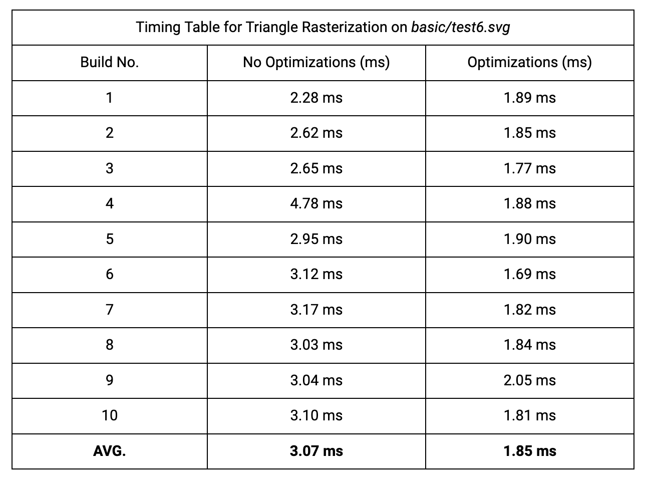
Due to our optimizations we improved cache efficiency and reduced the number of computations made per pixel.
The first optimization is in the sampling loop. By iterating through the $y$ coordinate values in the outer loop and the $x$ coordinate values in the inner loop, we improved the cache efficiency of our algorithm since a point $(x,y)$ maps to
The second optimization minimizes the number of computations needed per pixel. Instead of calculating $L_i(x,y)$ 3 times for every sample point (6 multiplications and 15 subtractions) we simply add $L_i(x+1,y)-L_i(x,y)$ or $L_i(x,y+1)-L_i(x,y)$ to our existing line function edge values depending on which loop we're in (inner and outer, respectively). We can pre-compute these 2 values for each of the three different edge functions $L_{01}$ , $L_{12}$ , and $L_{20}$ (6 constants). For example, given a counterclockwise triangle the value we would add to $L_{01}$ for every x-shift is $dX(y_0-y_1)$ or simply $y0-y1$ since $dX=1$ in this case. Using this method we can reduce the amount of work per pixel to just 3 additions.
|
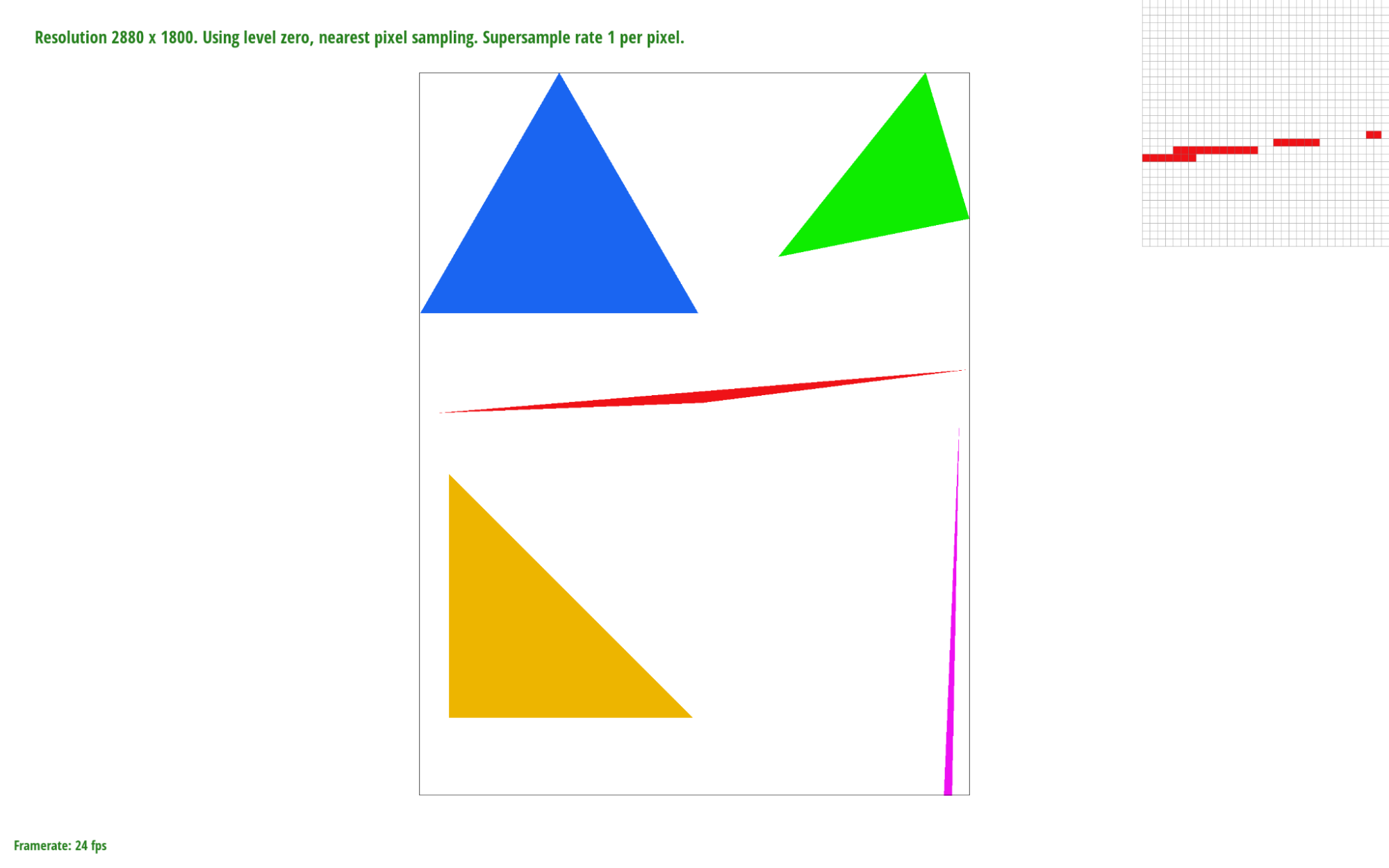
Our supersampling algorithm samples $N$x$N$ sub-pixels for every pixel in screen space, where $r_{sample}$ is the sample rate and $N=\sqrt{r_{sample}}$. For every x-shift within the pixel area we add $L_i(x+2OS,y)-L_i(x,y)$ to our edge values and for every y-shift we add $L_i(x,y+2OS)-L_i(x,y)$. Here $OS$ represents the offset, calculated as $\frac{1}{\sqrt{r_{sample}*2}}$, that gives us the center of a sub-pixel when added to its x and y coordinates. This means that the distance between two sub-pixels is $2OS$.
If a super sample passes the point-in-triangle test, we set
Then, in
Fig. 1.2

|
|

|
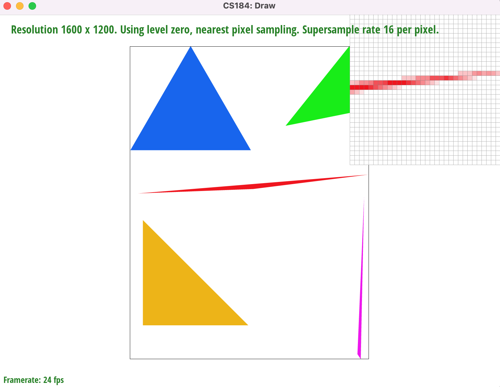
Supersampling minimizes image aliasing artifacts, such as the jaggies and gaps on the rightmost corner of the red triangle, by attenuating high image frequencies through convolution (In this case we achieve this using a 1-pixel box filter). By sampling the centerpoints of sub-pixels we can fill in pixels whose area is only partially within a given triangle, not including the centerpoint (such as the corner of a pixel). It also gives us a set of $N$x$N$ RGB values which we can average together and use to color pixels that border or intersect triangle edges. This helps smooth out the transitions between the red pixels and the white background. According to the Nyquist Theorem, we get no aliasing from signal frequency signals that are less than the Nyquist frequency (half the sampling frequency). Therefore by increasing our sampling frequency from 1 sample per pixel we are increasing the Nyquist frequency and diminishing aliasing at the higher image frequencies (i.e sharp changes in color or triangle edges)
|
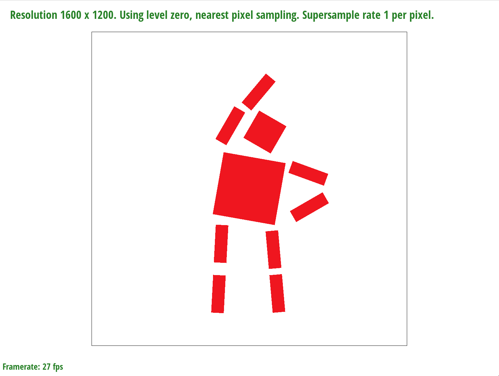
In order to achieve the desired pose in Fig. 1.3 we used a series of rotations on the arms, legs, head, and torso. We also used translation on the sub-parts of each limb to make it appear as though the robot's left arm and leg are slightly stretched.
|
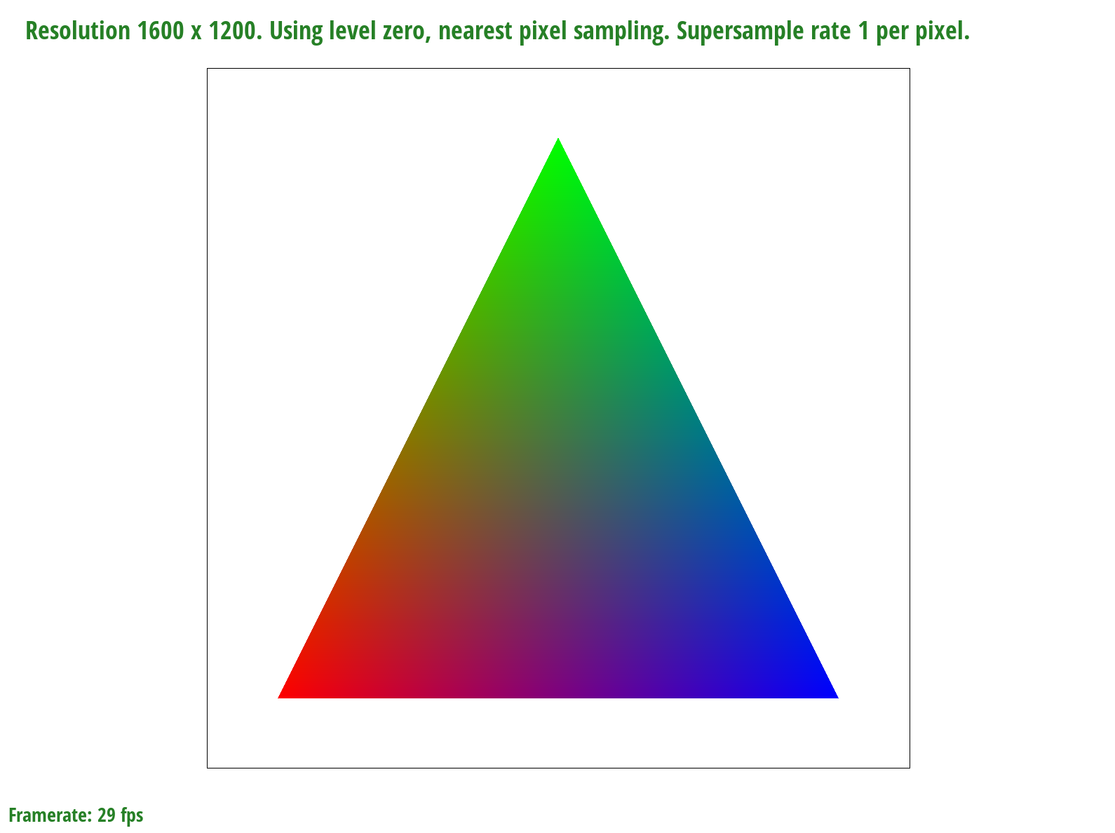
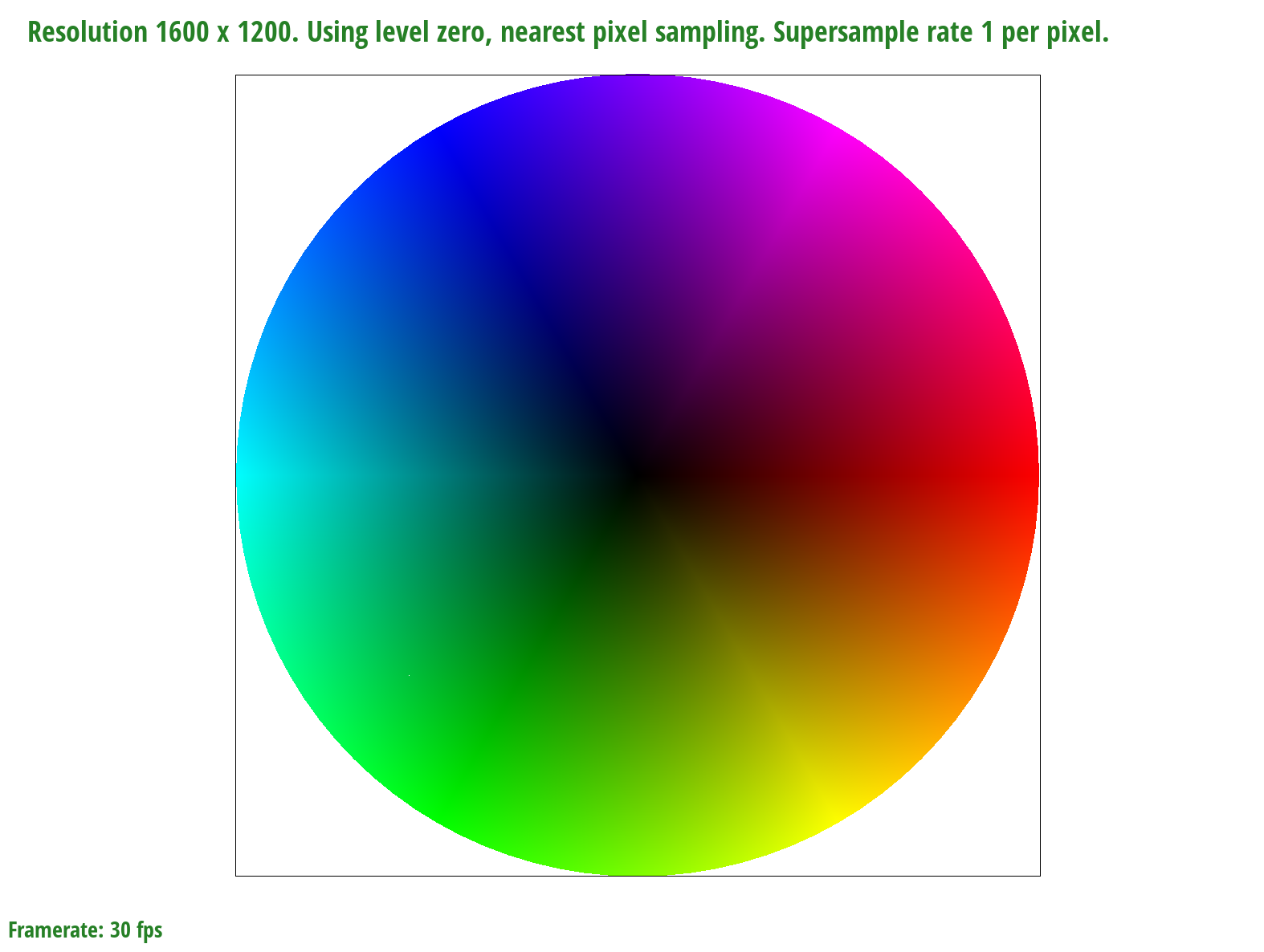
A barycentric coordinate system allows us to express any point located within a triangle as a weighted sum of $V_A$, $V_B$, and $V_C$ ($V = αV_A + βV_B + γV_C$) which can represent a number of things such as position, texture coordinates, color, normal vectors, material attributes and more. The constraint we must follow is that the scalar values $α$, $β$, and $γ$ must add up to one. Each scalar value can be calculated by finding the ratio of the perpendicular distances from the edge that sits opposite the vertex it scales to the vertex it scales and the desired point within the triangle. For example, α = $\frac{L_{BC}(x,y)}{L_{BC}(x_A,y_A)}$. Thus, barycentric coordinates allow us to linearly interpolate values within a triangle.
|
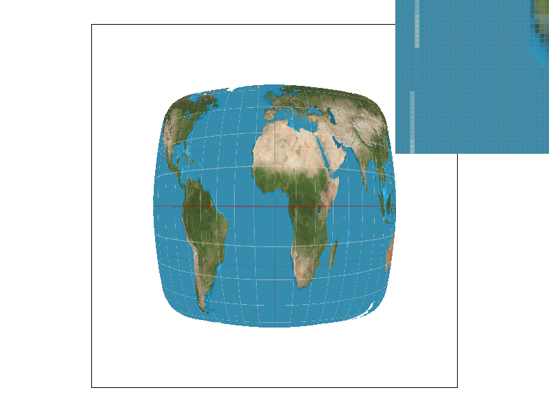
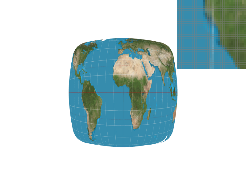
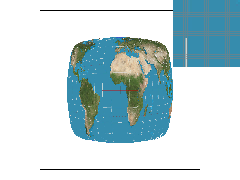
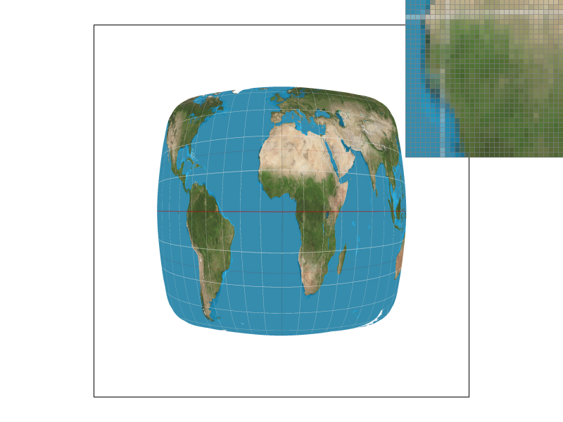
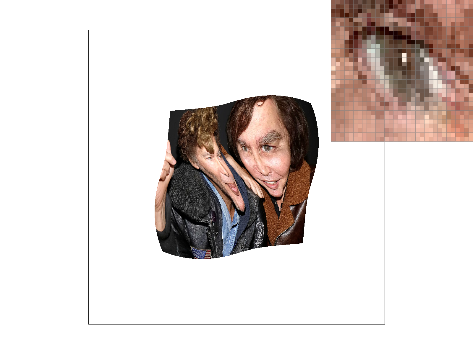
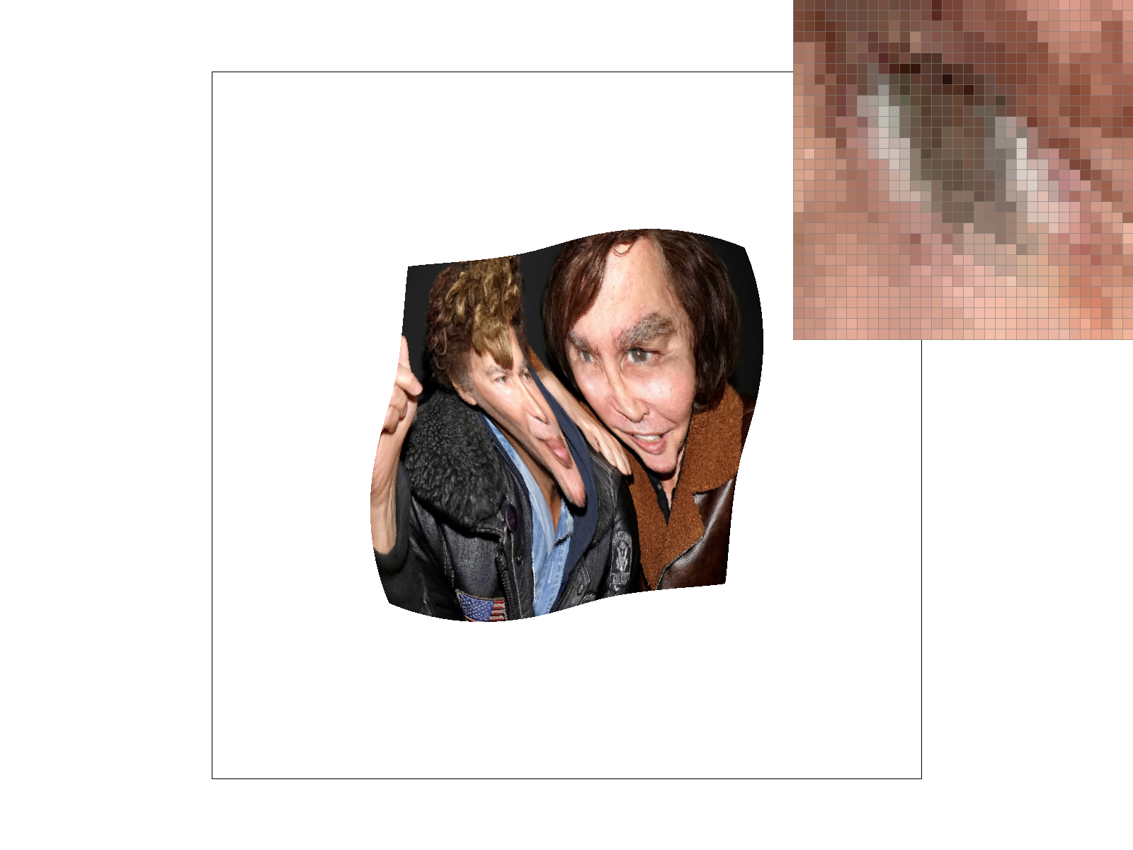
We can only sample at specific intervals so if we want a point in between where we sampled, we need to use the data from sampling to generate data that can represent that in-between value. We implemented two methods of sampling, nearest and bilinear. Nearest sampling makes the in-between point take on the color of the nearest of the 4 nearby points by rounding the coordinates and clamping. Bilinear sampling first creates two colors on the two horizontal interpolated lines of the 4 points that have the same $x$ value as the sampled point, then we use those two colors to get a linear interpolation for the sampled point, as demonstrated in lecture. We use texture sampling when the image gets distorted due to texture mapping so that we can get a color for a distorted surface even though our viewing angle of that surface has changed.
|
|
|
|
We see that the bilinear images have much smoother white lines on the distorted map that appear less jagged. This is because even though the pixels that make up the lines in the bilinear images are not truly fully white, they appear white in the whole image and it makes the line look smoothed out while in the nearby sampling method, the pixels are either white (part of the line) or not. There is not really an in between, which makes the lines look more jagged because there is no blurring. In general, there will be large differences when there are very small/thin and/or long continuous smooth curved lines because nearest will make those look jagged while bilinear will blur them a bit to make them look smooth.
Level sampling uses mipmaps to generate different qualities (“levels”) of a texture before it needs to be used, then when a texture is distorted, areas that are further away can use a lower quality texture. We implemented level sampling for texture mapping by passing in $uv$ coordinates that were acquired using barycentric coordinates and linear algebra and the differentials that are used to compute what mipmap level would be appropriate. We then get the difference between the differential and the actual vector, scale it according to the width and height of the full size texture, and then take the max of both norms, then return the log base 2 of that as the initial value for the level. We check what
Increasing the samples per pixel increases memory usage and reduces speed, but smooths lines and reduces rendering artifacts. The nearest pixel sampling is faster and requires less memory and bilinear sampling, but it results in more rendering artifacts (jaggies). Level sampling reduces memory usage by using lower quality and therefore sized textures and reduces graphical artifacts like aliasing but it blurs the image which may be undesirable.
|

|

|
|