CS 184: Computer Graphics and Imaging, Spring 2023

Project 3-1: Path Tracer

Tyler Bhadra, Victor Zhang

Overview

For this project we implemented the core routines of a physically-based renderer that uses a path-tracing algorithm. The first of these core routines was ray-scene intersection, which allowed us to calculate intersection points between camera rays and objects in the scene. The second was acceleration structures, such as the bounding volume hierarchy which minimized the number of ray intersections we had to compute, speeding up rendering time significantly. The third and fourth were direct and global illumination calculations, using Monte Carlo integration and various sampling methods, for more realistic lighting. The last was adaptive sampling which optimized the number of samples taken per pixel by checking for convergence.

Part 1: Ray Generation and Scene Intersection

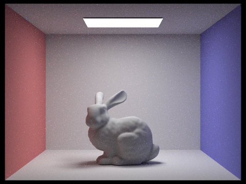
A physically-based renderer relies on the physical model of light which describes light as rays that travel in straight lines from light sources (such as light fixtures or the sun), bouncing off of objects in the world into our camera lens. Modeling scenes in this way allows us to get very realistic renderings of images. However, computing lighting calculations for every conceivable ray in our scene and figuring out which ones reflect back into our imaginary camera would be impossible to properly and efficiently implement.

To solve this, we can model light as a ray (Vector3D) that we shoot out from our imaginary camera lens through each pixel of the image plane and out into the scene. This allows us to trace shadow rays from hit points to test for light visibility, then fill in that particular pixel with a color value that is weighted by the calculated lighting contributions along our camera ray.

To do this we can take points from each pixel in image space (The coordinate system for the image) and project them into camera space (The coordinate system for the camera) using a series of translations and scales. If we multiply this point in camera space by the camera-to-world rotation matrix we can project the camera space point (the point we shoot the ray through from the camera origin) out into world space (The coordinate system the whole scene uses). From here we can test the camera ray for intersection with objects that are situated in the scene. This is achieved by solving for intersection points using the ray equation (r(t) = o + td, 0 ≤ t < ∞), plane equation ((p - p') • N = 0), and other equations for primitive objects such as spheres ((p - c)² - R² = 0).

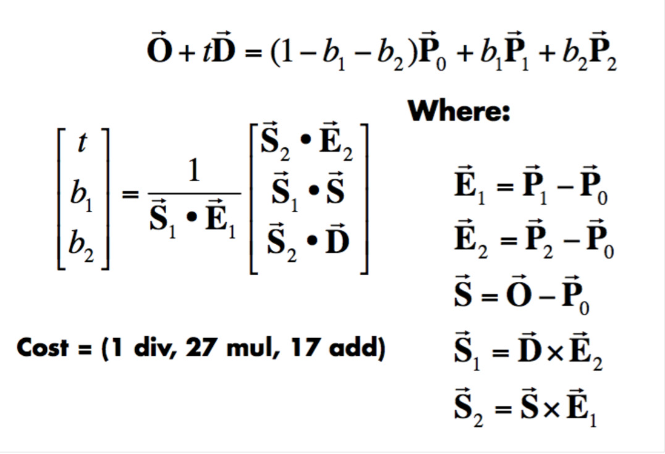
In order to test a ray for intersection with a triangle we used the Möller Trumbore algorithm, as shown below:

This allows us to express the plane intersection point of a ray as a set of barycentric coordinates for the triangle (P₀, P₁, P₂) within that plane, where α = 1 - b₁ - b₂, β = b₁, and γ = b₂. Therefore, if t lies between min_t and max_t of our ray (Which represents the "beginning" and "end" of the ray segment), and α, β and γ all lie between 0 and 1 then we know that this ray intersects with this particular triangle. For each intersection we store the t-value of the input ray where the intersection occurs, the surface normal at the intersection (which we calculate by interpolating the vertex normals of the triangle n₁, n₂, and n₃ using the above barycentric coordinates), a pointer to the primitve itself, and lastly a pointer to the Bidirectional Scattering Distribution Function (BSDF), or surface material, of that primitive.

Part 2: Bounding Volume Hierarchy

Our recursive BVH construction algorithm takes a set of primitives from the scene and initializes a BVHNode with a bounding box, bbox, that encapsulates them. Once the node is initialized, we check that the number of primitives in this node is at most max_leaf_size. If it is, we know that we've reached a leaf node and can terminate the recursion. If not we partition the node along the widest dimension of the bounding box at the average centroid point of all the primitives in the node. Then we do an in-place sort on the set of primitives by their centroid point along the partitioned axis. This allows us to store all the primitives of the left node before the primitives of the right node, letting us define each child by recursing on the left and right halves of the set of primitives.

After implementing the Bounding Volume Hierarchy (BVH) we were able to render scenes significantly faster than when we were rendering them with the naive method of exhaustively testing for ray intersections with every single primitive. For example, without the BVH cow.dae took 301.57s to completely render (~5 minutes). With the BVH, it took only 0.1363s to fully render. Larger files like CBLucy.dae were practically impossible to render on our local machines without the BVH. Partitioning the primitives into a hierarchical tree structure of bounding boxes allows us to efficiently traverse the spatial area of the scene in order to find the small set of primitives actually intersected by a particular ray in logarithmic time. This is because we can ignore entire collections of primitives if the ray of interest does not intersect with the bounding box of a BVHNode. This let's us avoid a very large number of unecessary computations for primitives that the ray never intersects.

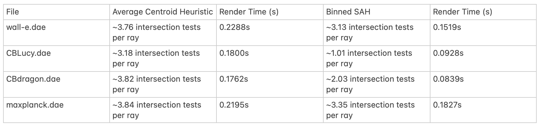
In order to more optimally partition nodes in the BVH we utilized a binned surface area heuristic during BVH construction. Essentially, we split each node's bounding box into B uniform partition planes which define B - 1 canonical ways of splitting the set of primitives into two halves. For each of these possible partitions we evaluate the SAH value as C_trav + SA(L)*prim_count_left + SA(R)*prim_count_right, where C_trav is the ratio of the cost to traverse the BVH to the cost of intersecting a primitive, and SA(node) is the surface area of a node's bbox. We repeat this process for each axis and choose the partition which incurs the least cost. (For our implementation we used B = 32)

With this new heuristic we made marginal improvements to rendering speed, but were still able to reduce the number of intersection tests per ray. This reduction is more significant for files where there is a more uneven distribution of primitives (i.e. odd geometry, more protrusions, etc...) like CBLucy.dae where there is more to be gained from making smart partitions as we can reduce the amount of empty space included in the bounding boxes of nodes, letting us ignore nodes which we would have otherwise had to explore if we used a worse heuristic (i.e. Nodes we need to check in situations where the ray intersects the bounding box, but still misses all of the primitives contained within).

Part 3: Direct Illumination

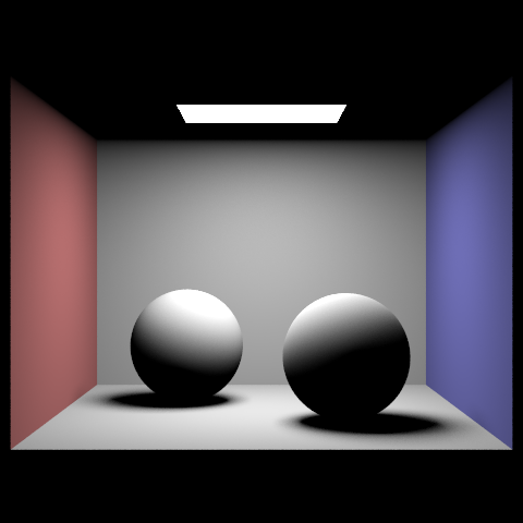
For Uniform Hemisphere Sampling, we first get a direction vector uniformly at random from the hemisphere coordinate system for the hit point. We take that vector and change it to the world's coordinate system and create a ray that can be tested for intersection against the bounding volume hierarchy. If it intersects, we get the emission of the intersected object, the BSDF of the hit point, and the cosine angle of the hemisphere sample. We multiply these together and add these according to the Monte Carlo estimator and repeat this process until we have the desired number of samples. After all the samples have been taken, we can account for the constant PDF (2π) by multiplying by the PDF and then we return the result divided by the number of samples taken.

For Light Importance Sampling, we go through every light in the scene. Point lights are sampled once whereas area lights are sampled ns_area_light times. Each time we sample a light, we call its sample_L function that returns its radiance given the hit point, while also giving us the direction between the light and the point, the distance between the two, and the pdf. We use the direction to create a ray and use that ray to check for intersection in the BVH. This time, we want to see that the ray doesn't intersect anything at all between the light and the point. If it does, the point is in the shadow of the light. Otherwise, we get the BSDF of the point and the cosine of the angle and multiply this together with the radiance and divide by the pdf. For area lights, we take all their radiances from the different samples and average them before adding. We add all of these samples together and return the sum.

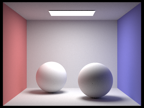
Uniform Hemisphere Sampling	Light Sampling

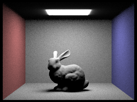
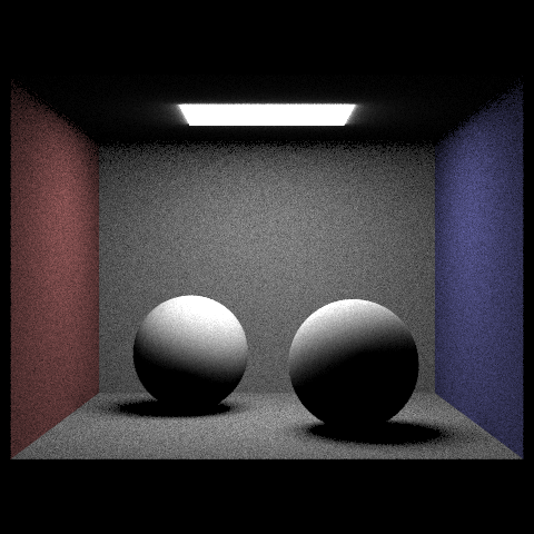
The changing number of light rays changes the number of samples we take of area lights. At lower counts, each point in space has noisier radiance due to the fact that if that spot samples an area of the light that isn't blocked and its neighbor samples a different area of the light that is blocked or has a different value for L_out then that results in noise. As the number of light samples increases, the noise decreases and even though we have a low number of camera rays per pixel, the brightess of each general area that a pixel would sample from is is pretty close in brightness due to the decreasing noise which makes allows for some of the smaller details of the dragon like the texture of its belly to be noticeable at higher numbers of light rays whereas it looks like a pixelated mess at 1 light ray.

The hemisphere sampling is noticeably more noisy than the light sampling due to the random nature of the sampling that can make the radiance vary wildly due to the randomness of where the ray lands. The only light in both scenes is the ceiling light so every spot's brightness will vary vastly from neighboring areas if it samples more of the light with its limited number of random samples. Light sampling only samples the lights for each spot instead of sampling random directions. Specifically, it samples different areas of the light. The noise seems to take form as spots being darker than they should be, which is why in the light sampling images, he scene as a whole seems brighter. The light also doesn't "bleed" through the edges in the light sampled images.

Part 4: Global Illumination

In order to implement indirect lighting we recursively bounced rays off of intersected surfaces. This lets us more accurately simulate the behavior of light rays which are reflected off of both illuminated and shadowed surfaces many times (rather than only from areas that are directly illuminated) before entering the camera. Thus, the gobal radiance reflected back into the camera is the accumulation of radiance measured at all of the reflected hit points of the inverse camera ray.

The bulk of our indirect lighting algorithm lies in the function Pathtracer::at_least_one_bounce_radiance which calculates the one bounce radiance of a ray in addition to the accumulated radiance from extra bounces. In this function we use Russian Roulette, with a cpdf of 0.7 to randomly terminate recursion before reaching the max recursion depth of max_ray_depth, which is a depth variable stored in the Ray object. For a particular ray, we first add the one_bounce_radiance to L_out, then sample a cosine weighted, hemispheric direction, w_in (We sample w_in since we are tracing inverse rays) for a new ray using the BSDF of the intersected primitive (Using DiffuseBSDF::sample_f). This also gives us a pdf as well as the reflectance value, bsdf_sample, which we will use later in our calculations. After this we check that the depth of this particular ray is greater than one, that the pdf is not equal to zero, and that we can recurse as dictated by the cpdf. If all of the above is true, we generate a new ray originating from the hit_pt of the current ray in the direction of w_in with a depth value one less than the current ray, then test for intersection with a scene object. If there is an intersection we recurse on this ray, scale the value of its returned radiance by our BSDF sample and a cosine factor, then divide by the pdf and cpdf.

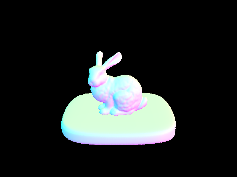
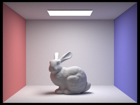
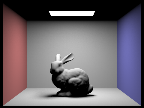
In the figure above, we see CBbunny.dae rendered once with only direct lighting, and once again with only indirect lighting.

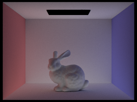
In the series of images above, we can see that increasing the ray depth increases the overall brightness of the image. Note that at ray depth = 0, the scene is rendered with only the zero bounce radiance. Similarly, at ray depth = 1, the scene is rendered with only direct lighting. At ray depths greater than one, indirect lighting is included.

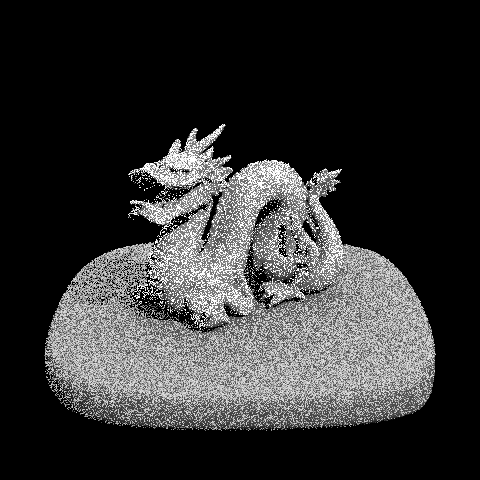
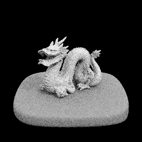
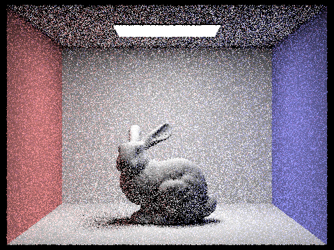
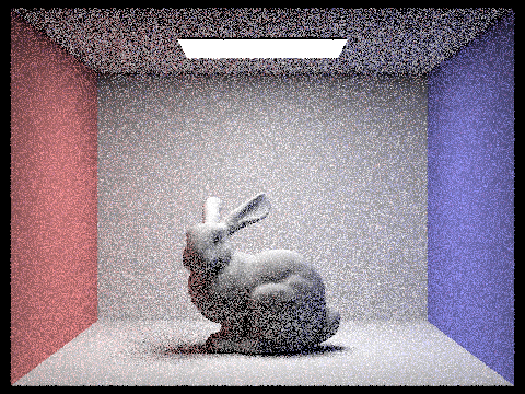
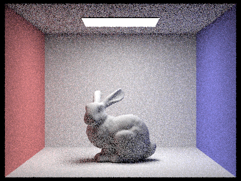
In the above series of images above, we can see that increasing the sample rate decreases the amount of noise in the image.

Part 5: Adaptive Sampling

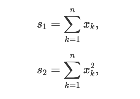
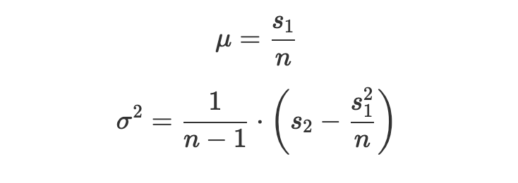
As shown above, in order to decrease the amount of noise in our renders we simply need to increase the sample rate. However, sampling at a fixedly high rate for every single pixel is not cost efficient, as some pixels converge earlier than others. Adaptive sampling solves this issue by letting us concentrate the samples on the most complicated parts of the image. To implement this we check for convergence every 32 samples using the convergence variable I defined as such:

In this case σ represents the standard deviation of our samples so far, while μ represents their mean. We can calculate σ and μ using values s1 and s2 which represent the sum of x_k and x_k², respectively, where x_k is the illuminance value of a sample.

By updating s1 and s2 at every sample we can immediately calculate σ, μ, and I. We know that a pixel has converged if the convergence variable I satisfies the inequality below:

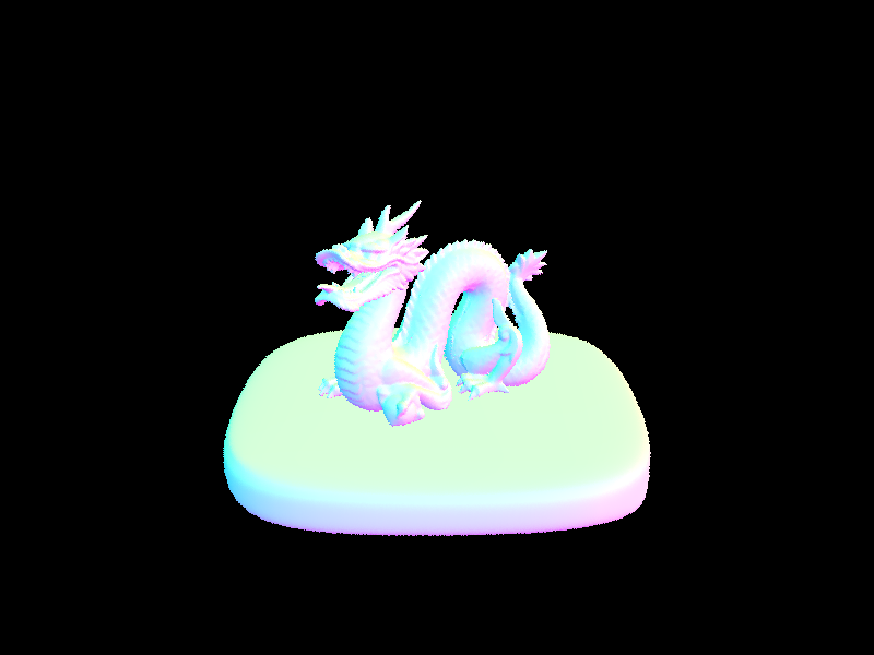
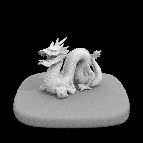
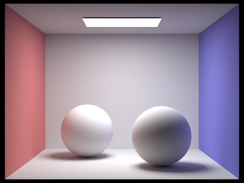
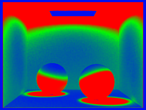
Once we've confirmed that a pixel has converged we stop sampling. Below are scenes that have been rendered with adaptive sampling. For these images we use a maxTolerance of 0.05. Red indicates a high sampling rate, while blue indicates a low sampling rate. Sampling rates are computed as the ratio between the actual number of samples and the maximum number of samples allowed.