Overview

In this project we were tasked with creating a program that modeled three dimsensional geometric objects. We achieved this by implementing bezier curves and surfaces by means of de Casteljau subdivision, as well as utilizing the halfedge mesh data structure to implement basic halfedge mesh operations, such as edge flips and edge splits, and loop subdivision.

Section I: Bezier Curves and Surfaces

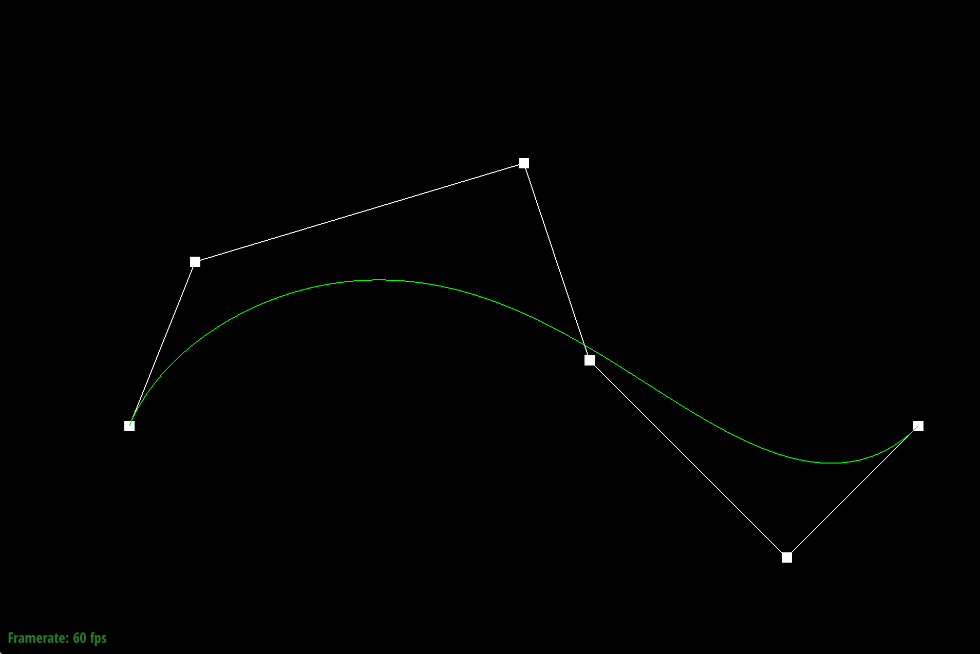
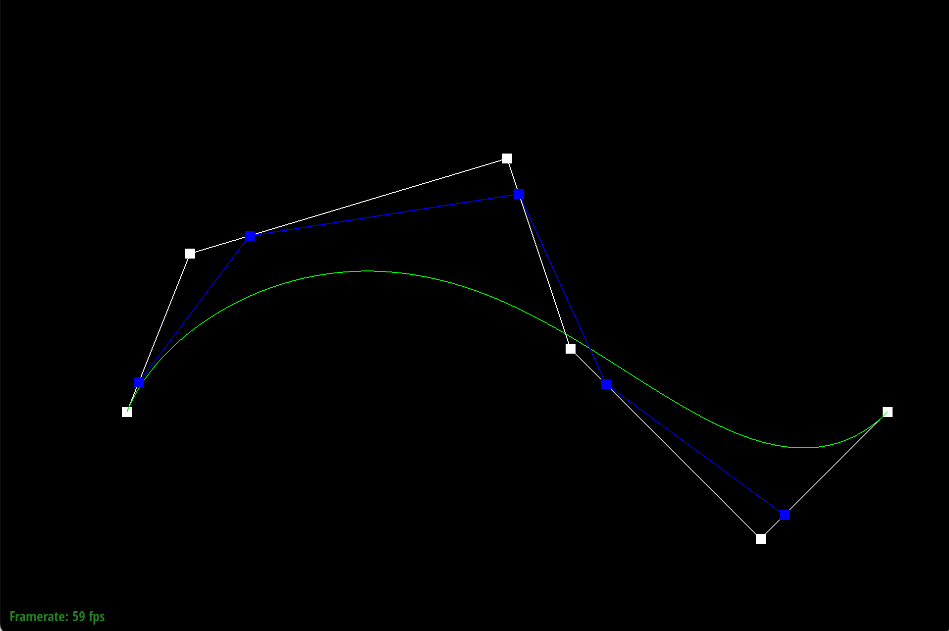
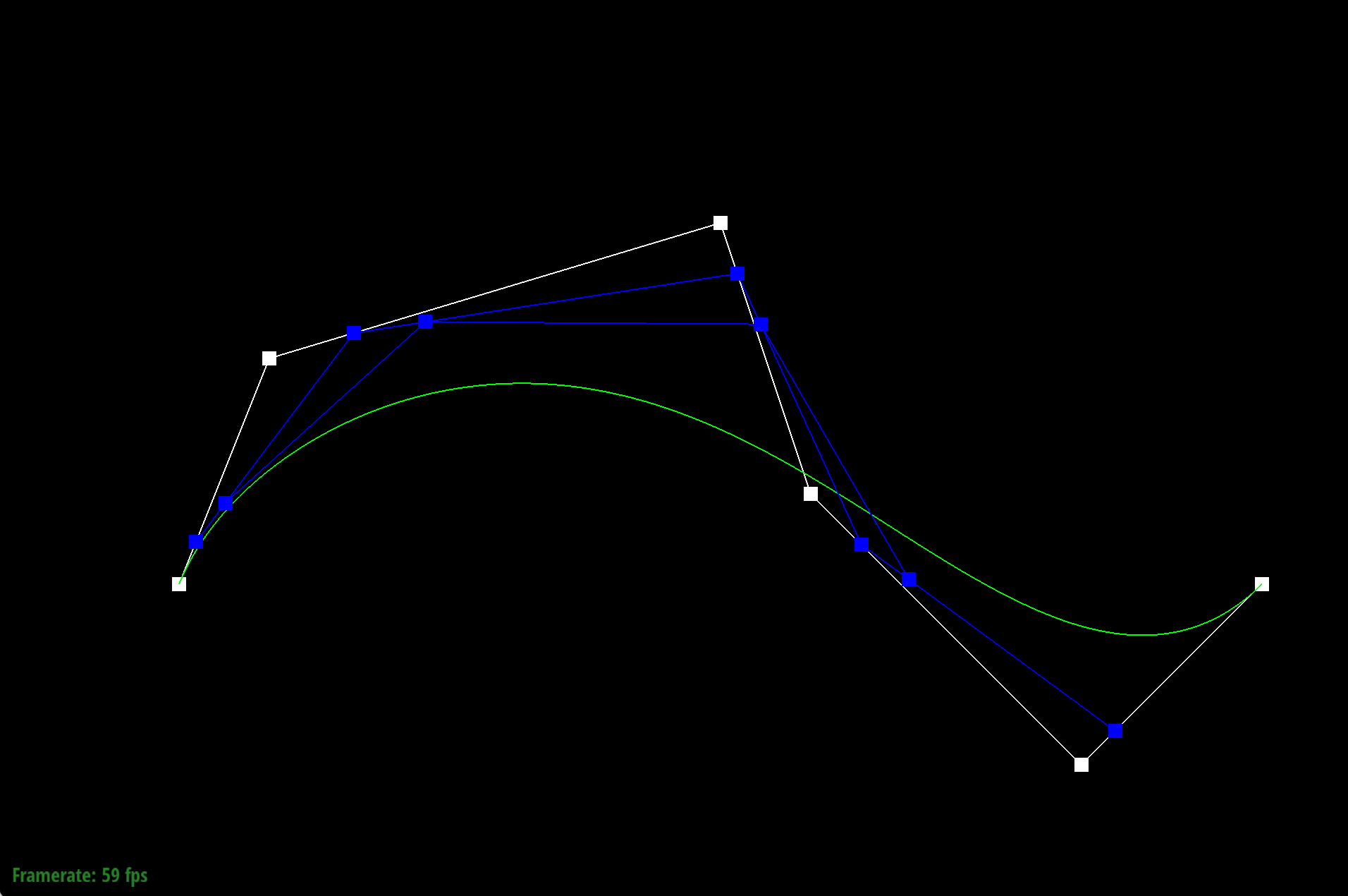
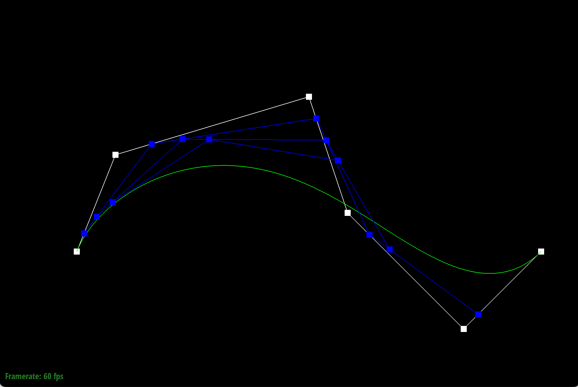
Part 1: Bezier Curves with 1D de Casteljau Subdivision

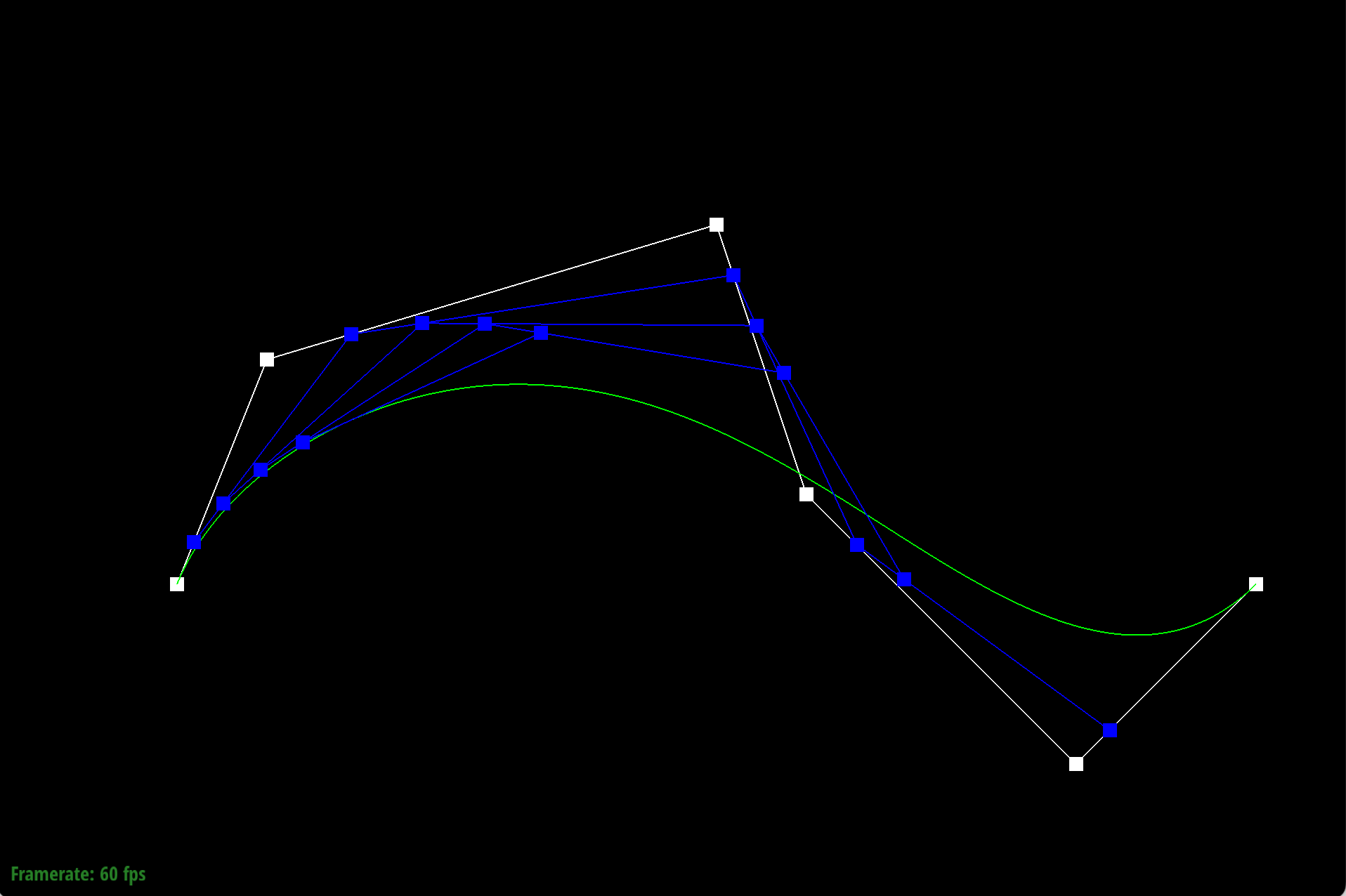
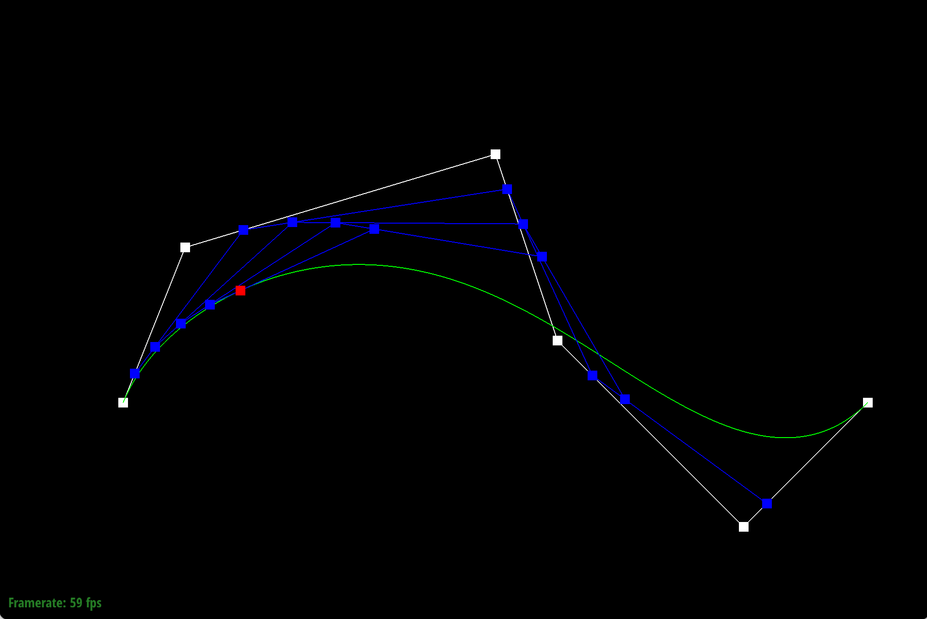
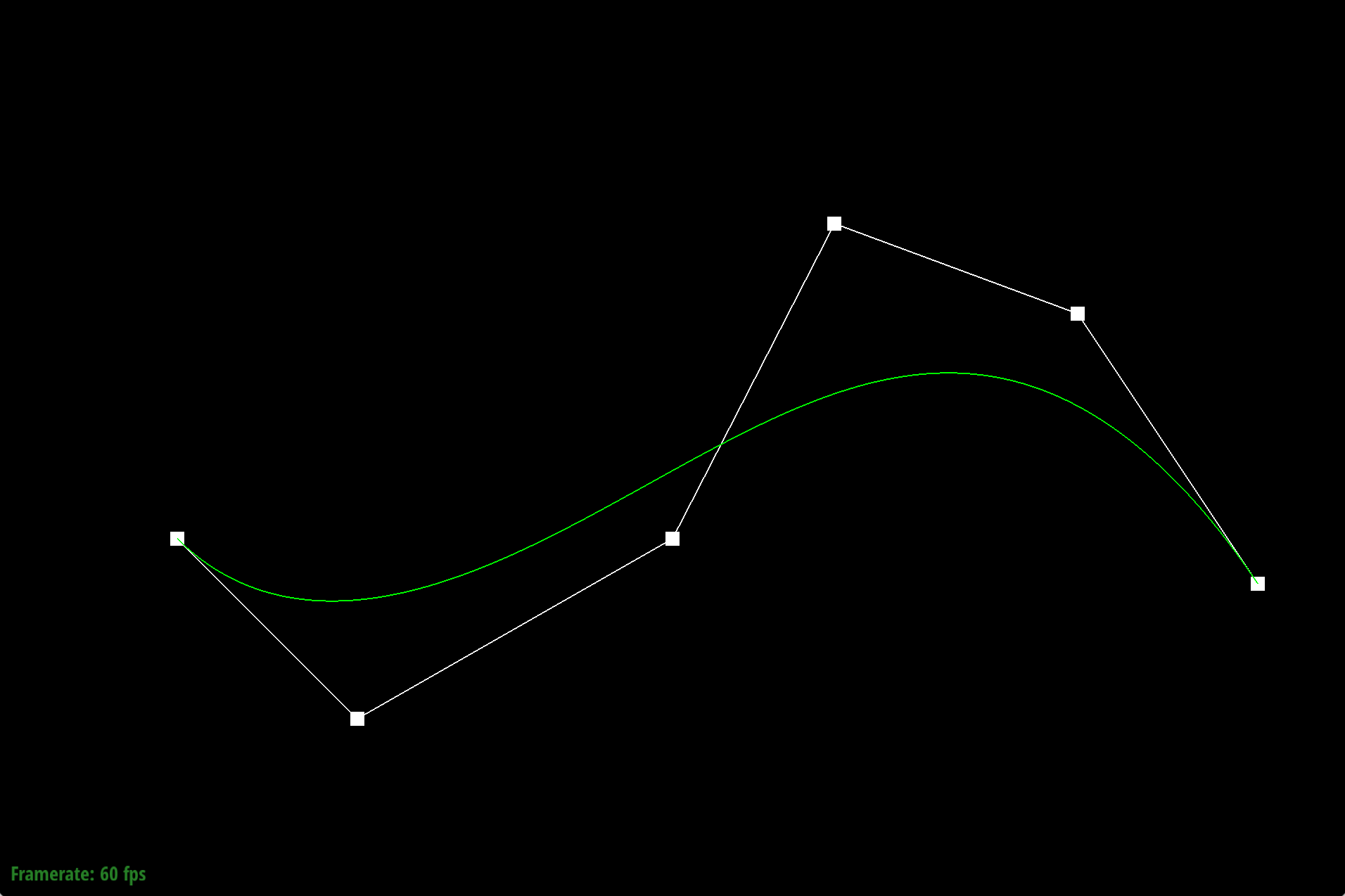
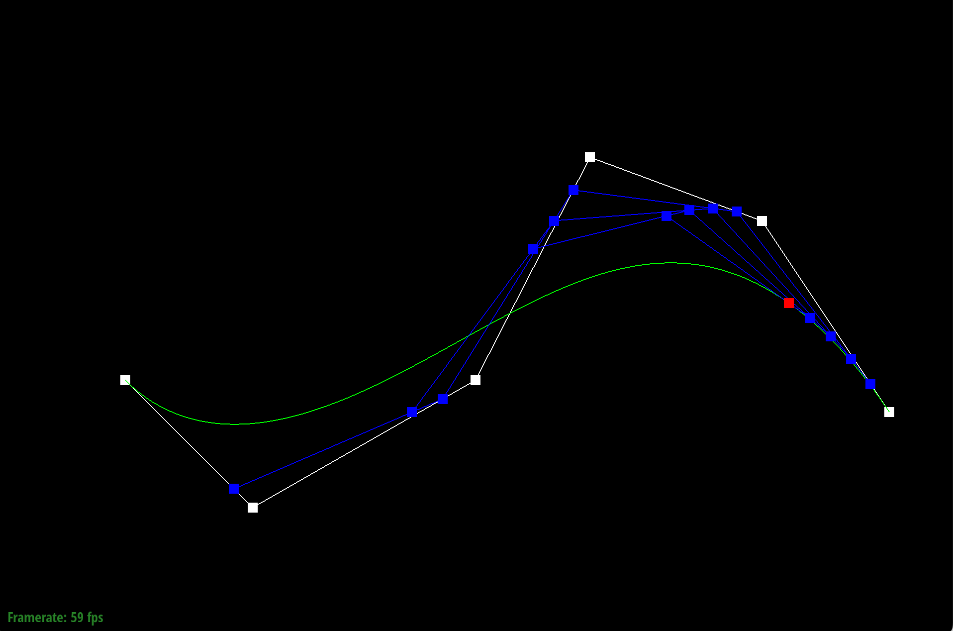
De Casteljau's algorithm allows us to find a single point that lies on a bezier curve uniquely defined by n control points at the parameter t. At each recursive evaluation step, we use linear interpolation to calculate n-1 intermediate control points at the parameter t, given the n control points (intermediate or otherwise) from the previous recursive step. For points p_i,...,p_n we can calculate intermediate points as such:

p_i' = lerp(p_i, p_i+1, t) = (1 - t)p_i + tp_i+1

Thus, by using De Casteljau's algorithm at many small increments of the parameter t (0.0 < t < 1.0) we can find as many points on the bezier curve as we want. This allows us to draw bezier curves given any set of control points in a very easy and simple manner.

Part 2: Bezier Surfaces with Separable 1D de Casteljau

De Casteljau's algorithm lets us evaluate points on a 1D bezier curve given n control points. In order to model 3D objects we can use bezier patches, which are surfaces with topographies created by a "net" of bezier curves defined by control points that lie along the x, y, and z axes. To evaluate bezier patches we can use De Casteljau's algorithm to evaluate points at parameter u on n 1D bezier curve "slices" of the surface across the z-axis. This gives us n control points which we can use to evaluate another point, at parameter v, on the bezier curve defined along the z-axis.

To implement this in code we iterated through the controlPoints vector, which is a member variable of the BezierPatch class, in order to evaluate points at u from each row of control points (Where each row is of type std::vector<Vector3D>). This gave us n control points for the "moving" bezier curve along the z-axis which we used to evaluate the final Vector3D point at parameter v. In other words, we evaluated the desired point (u, v) on the bezier patch specified by controlPoints.

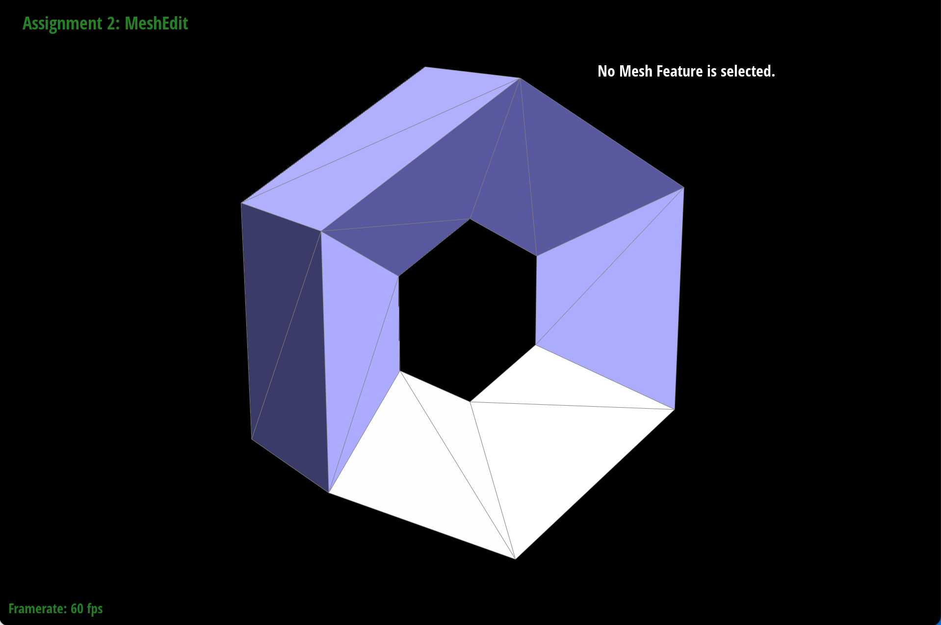
Section II: Triangle Meshes and Half-Edge Data Structure

Part 3: Area-Weighted Vertex Normals

Starting with the given vertex, we take the halfedge associated with it. We then iteratively take the next 2 halfedges to the get the other 2 vertices in that face, use the positions of the vertices to get 2 vectors of the face, then take the cross product to get a normal vector. We then add this normal vector to a vector that sums all the normals together and then since the cross product of these two vectors is twice the area of the face, the normal vector is already weighted by area. Then, we take the twin edge after my two previous next halfedges to go to the next face. If we ever hit a boundary, we go back to the halfedge of the vertex and go in the other direction (clockwise) until the boundary is hit again. Once all the faces are accounted for, we take the sum of all the normal vectors and normalize it to get a unit vector and return that.

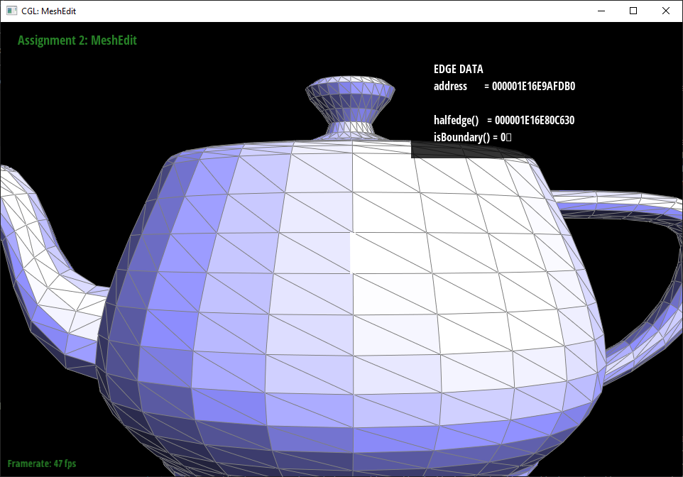
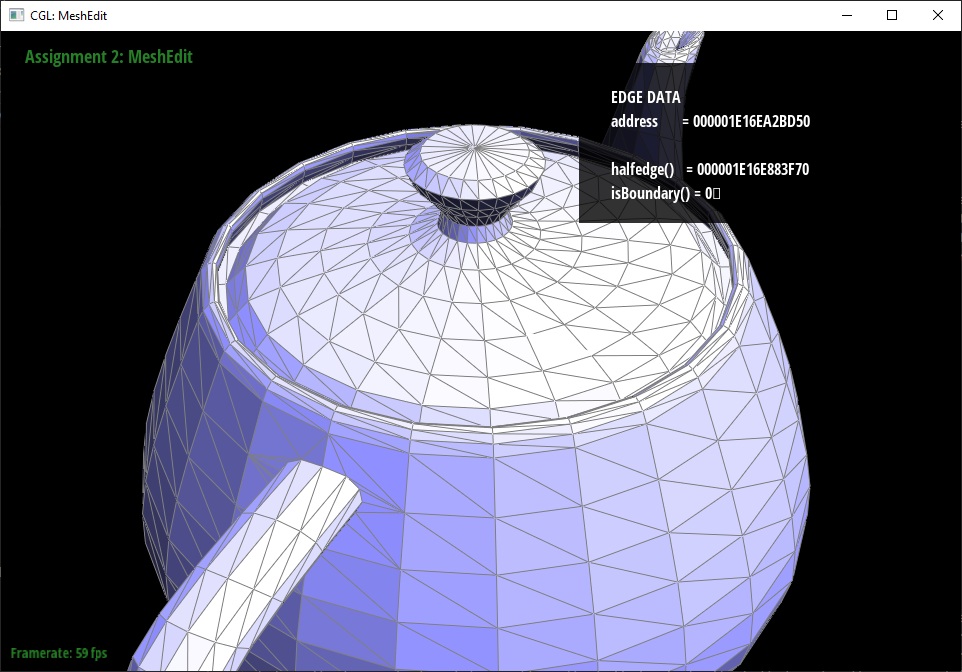
Part 4: Edge Flip

We first create variables for each element that needs to be tracked in the operation, so there are edges, vertices, halfedges, and faces all with appropriate names that denote what they correspond to on the given diagram on the spec. We then treat the bc edge as if it sort of rotated and became an edge from a to d and set all the halfedges of the vertices, faces, and edges accordingly. For all the halfedges, we redo their neighbors using setNeighbors according to what their new neighbors are on the spec diagram.

At first the program froze when we tried to flip an edge, but when we went back and went over every line in the edge flip function, it turns out that two of the halfedges were acquired incorrectly with the wrong mesh traversal operation order. It turns out that when pasting to avoid typing as much, we put the next operation before the twin, which ended up setting the halfedge to be the halfedge of either an unrelated face or a nonexistant face.

Part 5: Edge Split

Like in the edge flip operation, we first created variables for each of the existing elements. We renamed some of the existing elements that would be reused as another element that was replacing it (like how the vertex splits the edge into 2 edges so 1 of the edges can be reused) to reduce the number of new objects needed. Then we created the new objects that we still needed in the mesh. For the new vertex, we assigned it a position that was the average of the two vertices that it was bisecting. Then all the variables were updated with the two old faces getting mapped to two of the four faces after the split. The updates were much like in the edge flip operation.

This one actually worked on the first try since it was mostly based off of the edge flip and the edge flip operation was debugged before edge split was written.

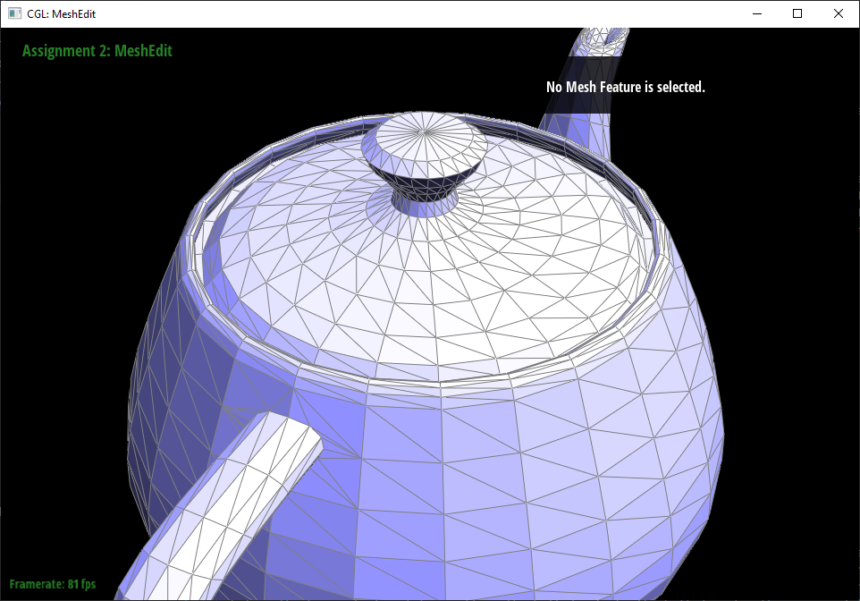
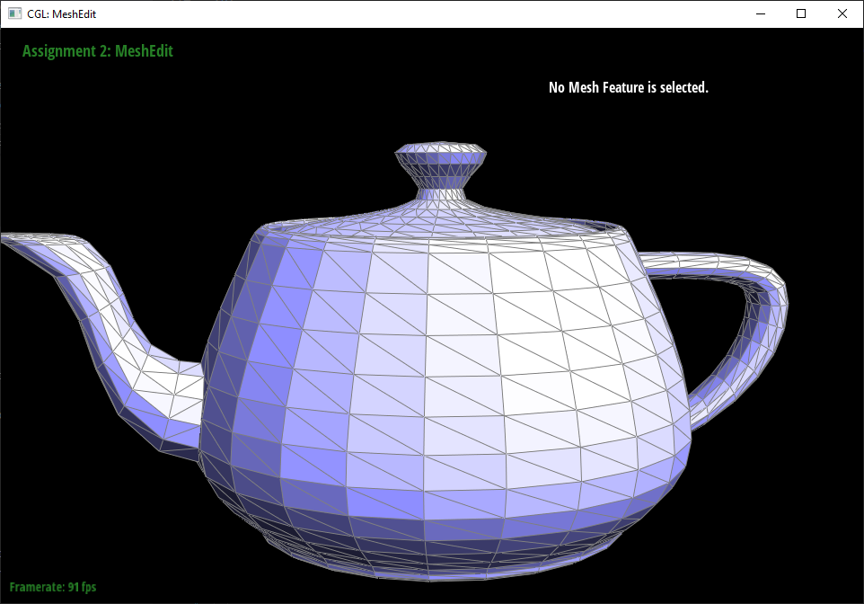
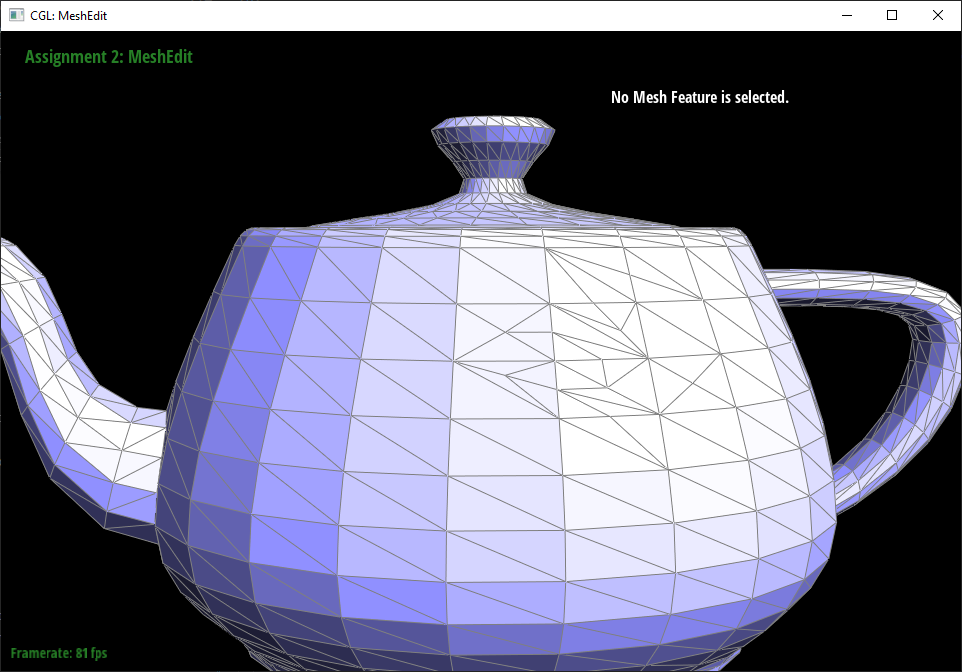
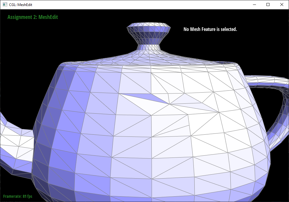
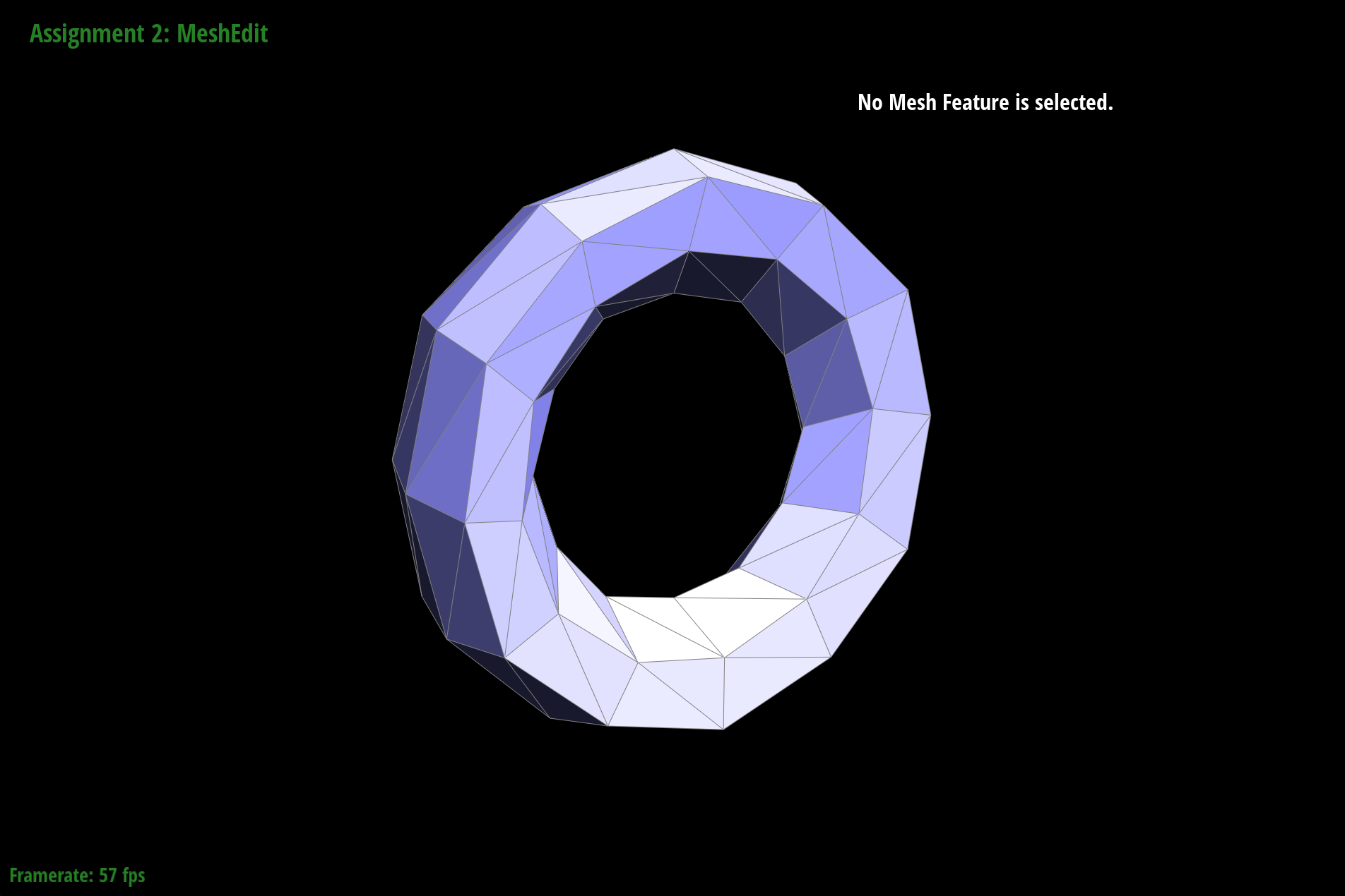
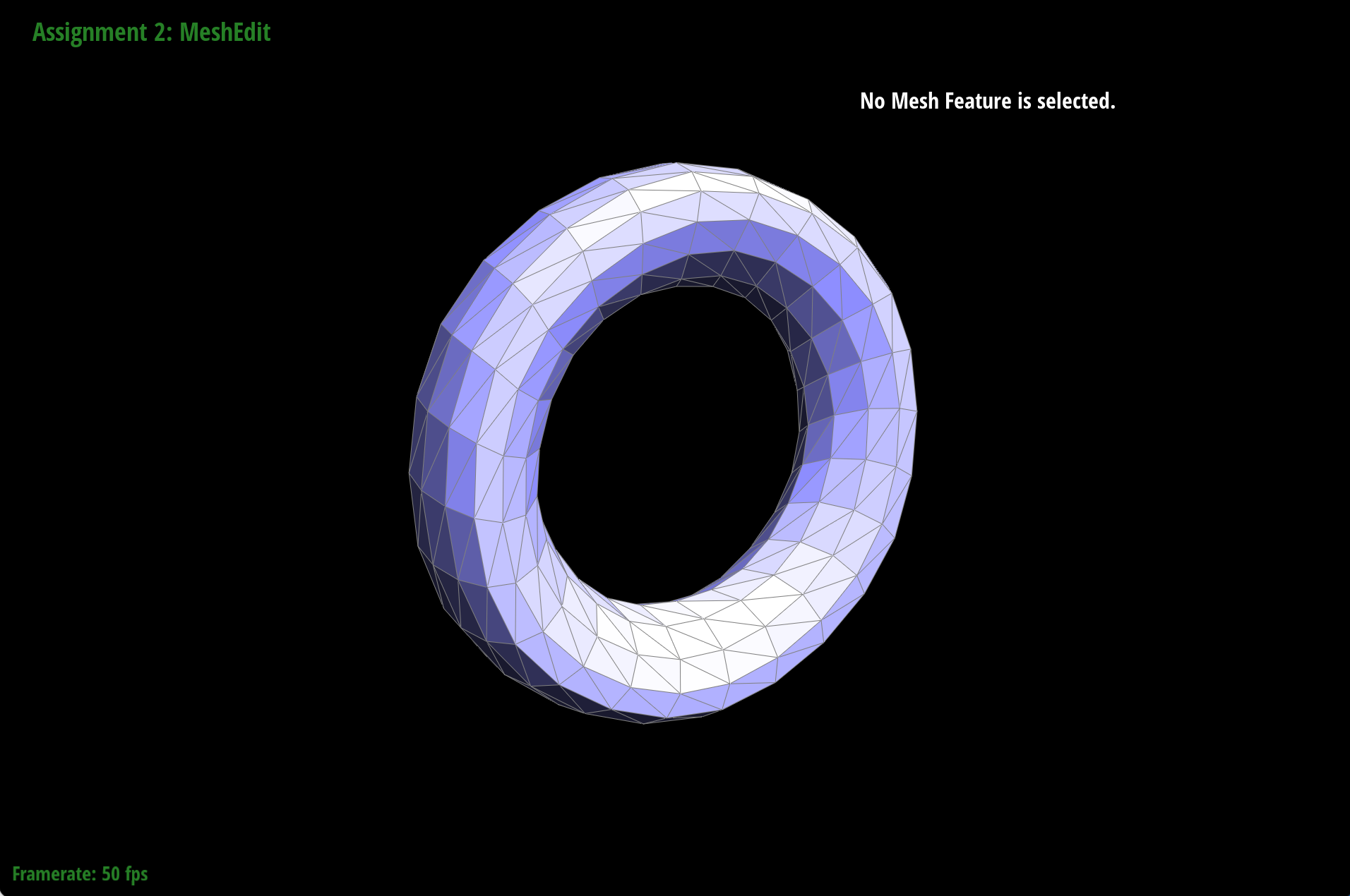
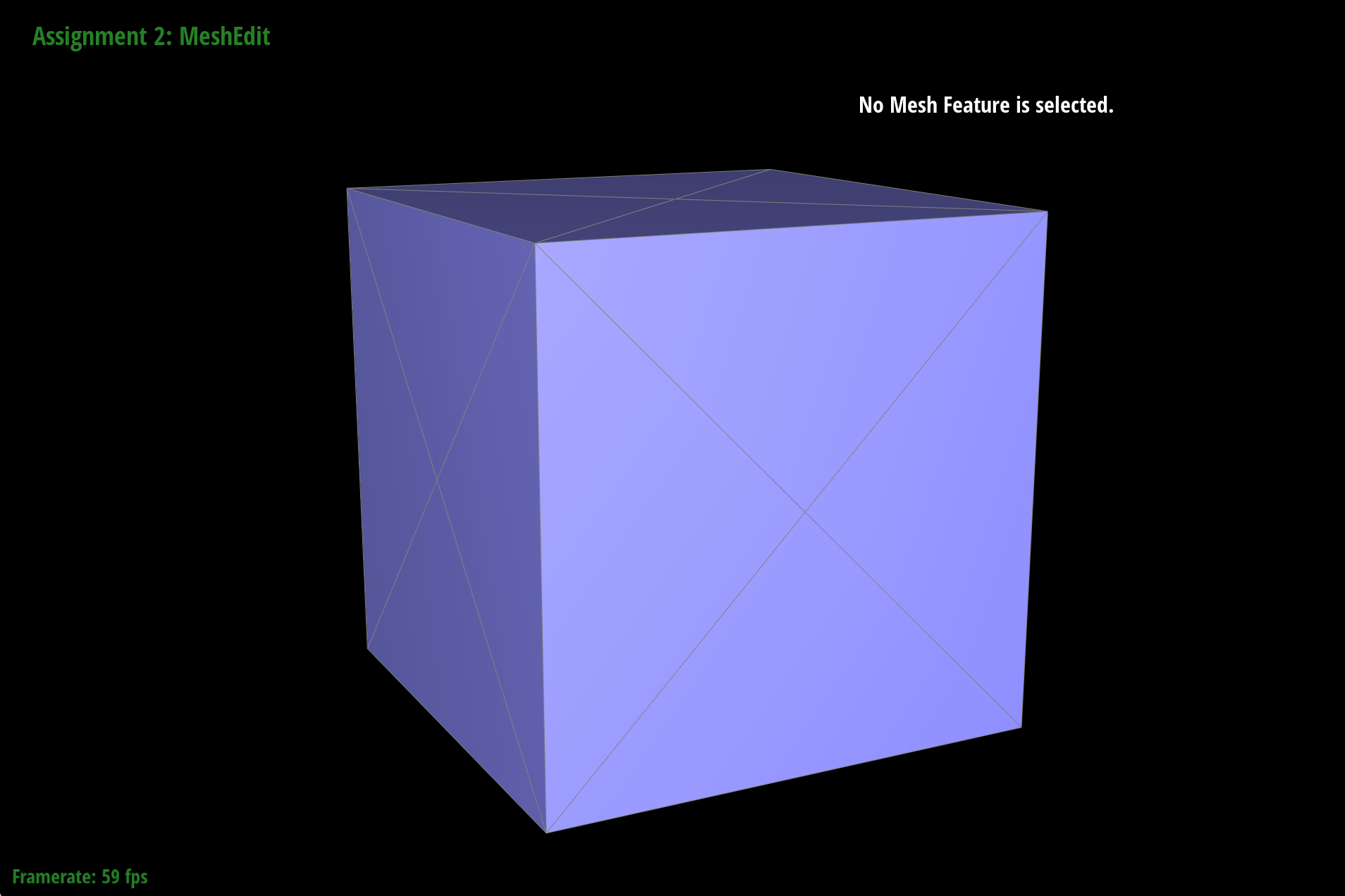
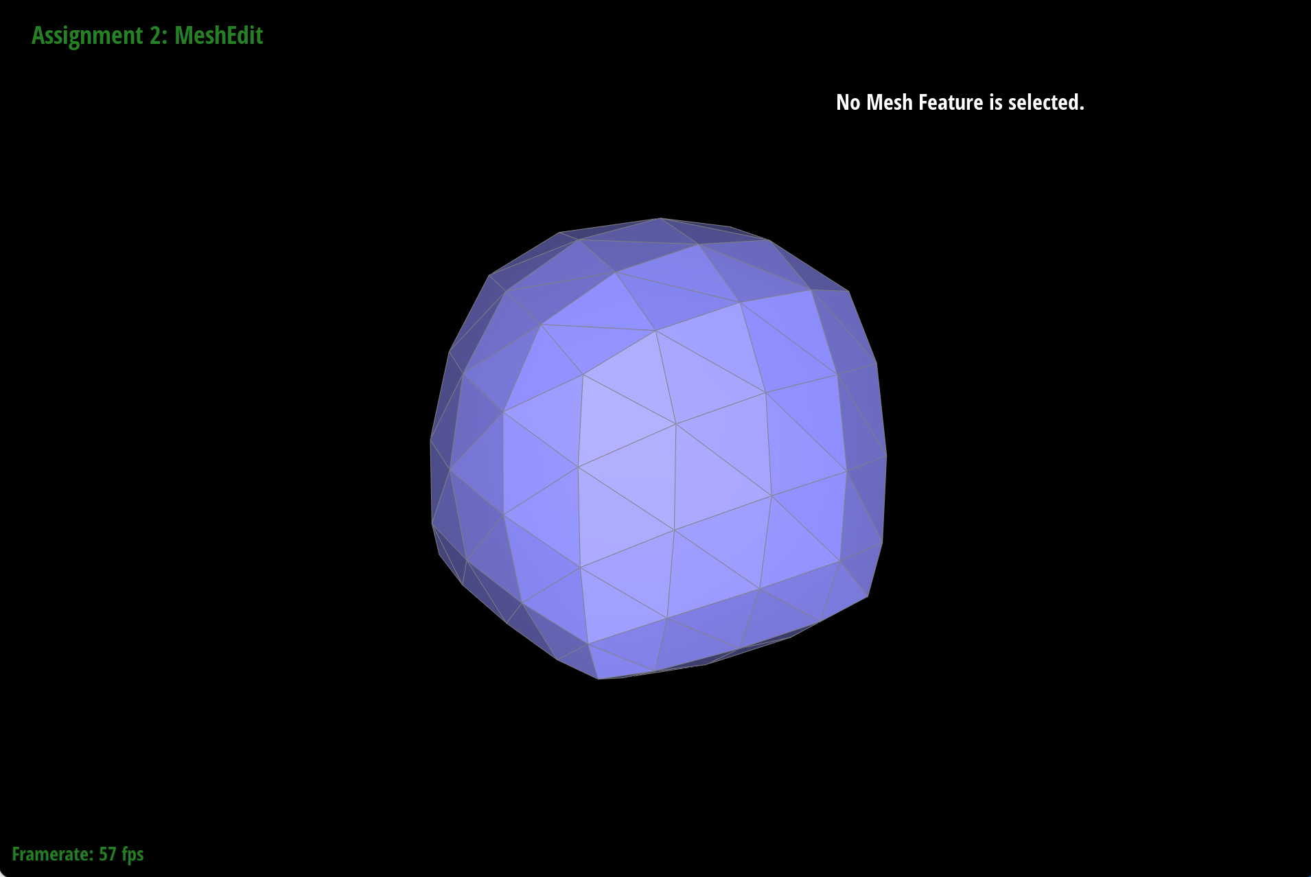
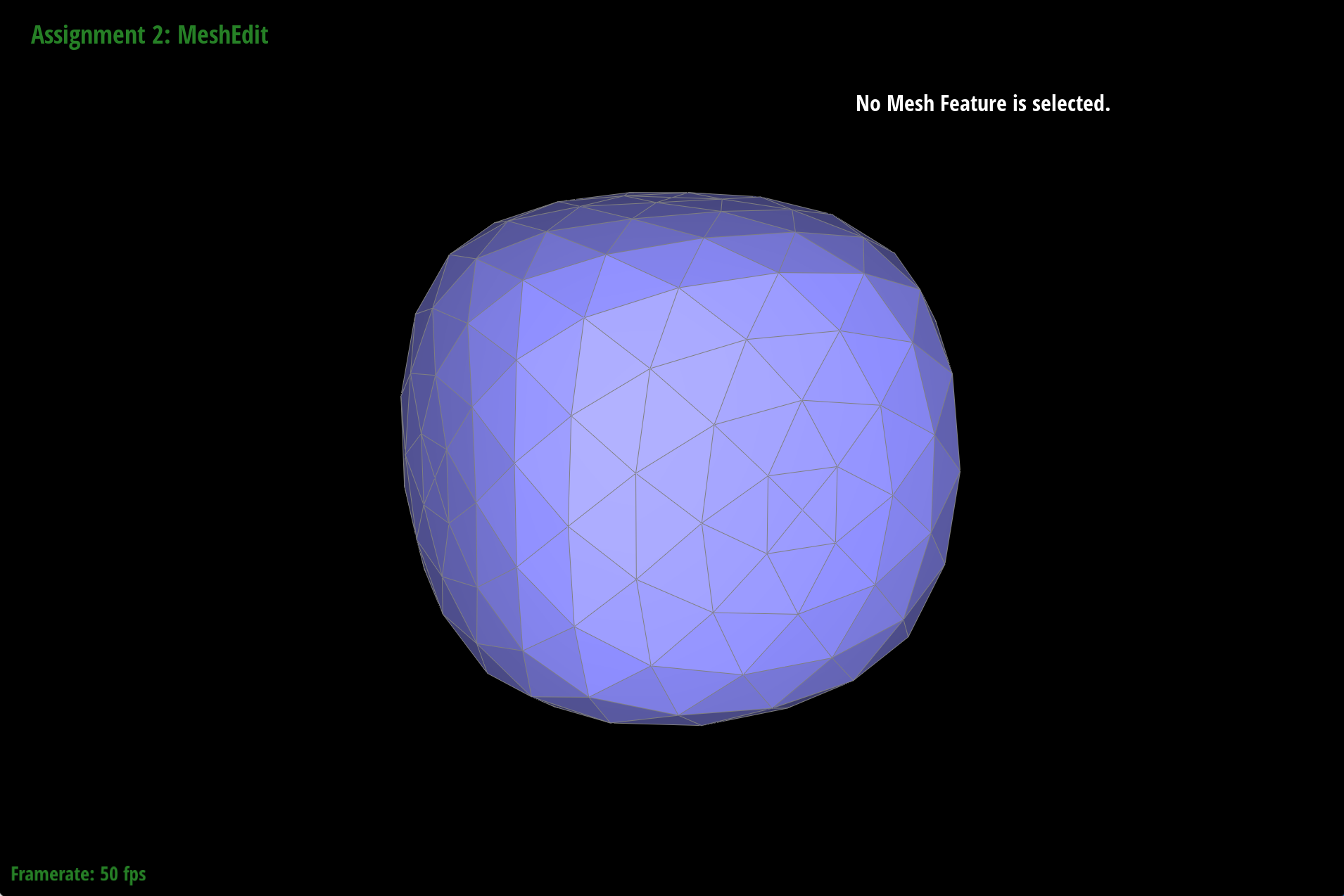
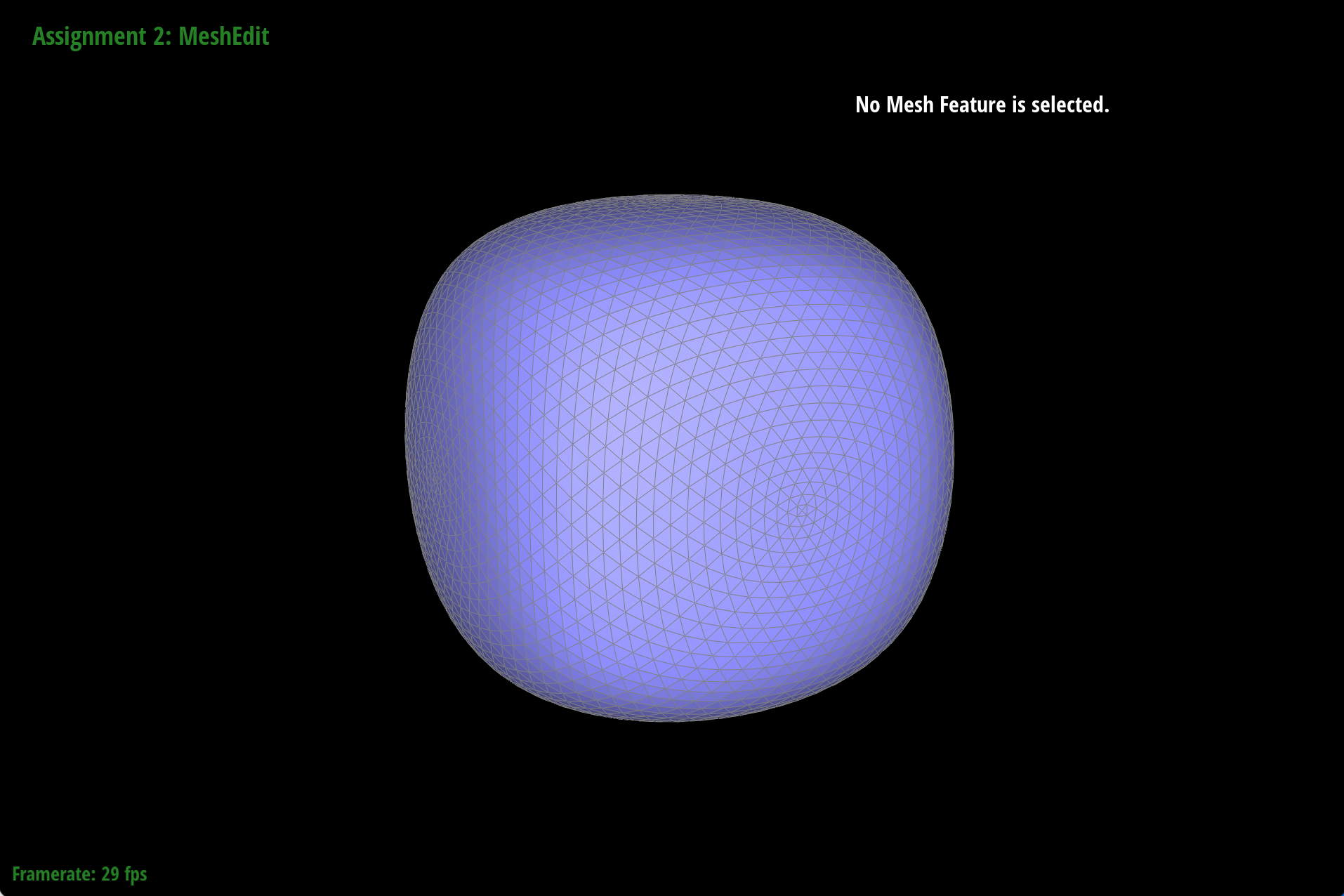
Part 6: Loop Subdivision for Mesh Upsampling

We implemented loop subdivision by following the steps described in the project spec. First, we calculated the new weighted vertex positions for both new and old vertices. For old vertices we stored new positions in the newPosition member variable of the Vertex class. For new vertices we stored new positions in the newPosition member variable of the Edge class. This way we could assign new vertices, that were created from edge splits, the correct new position by accessing the value through its incident edge.

We then split every edge from the original mesh by checking that both of the endpoint vertices for a given edge had false isNew flags (i.e old vertices as opposed to new vertices). After this we flipped every new edge connecting an old and new vertex. It is important to only flip new edges because old edges (such as the 2 edges that represent an edge after it has been split) already sit along the boundary of the 4-way subdivided triangles. Finally we finalized the position for every vertex by copying its newPosition value into its position variable.

After loop subdivision sharp corners and edges are smoothed and rounded out. We can reduce this effect by splitting edges before upsampling. This works because of the way the positions of old vertices are updated. Since the calculation of new positions includes a weighted sum of the original positions of neighboring vertices we can increase the number of incident vertices for any one vertex by pre-splitting edges. This increases the number of samples we use to estimate new vertex positions which in turn creates a softer curve or transition between high 3D mesh content frequencies (sharp edges and corners). Just as supersampling created smoother looking triangles, loop subdivision increases the consistency of the mesh as we upsample.

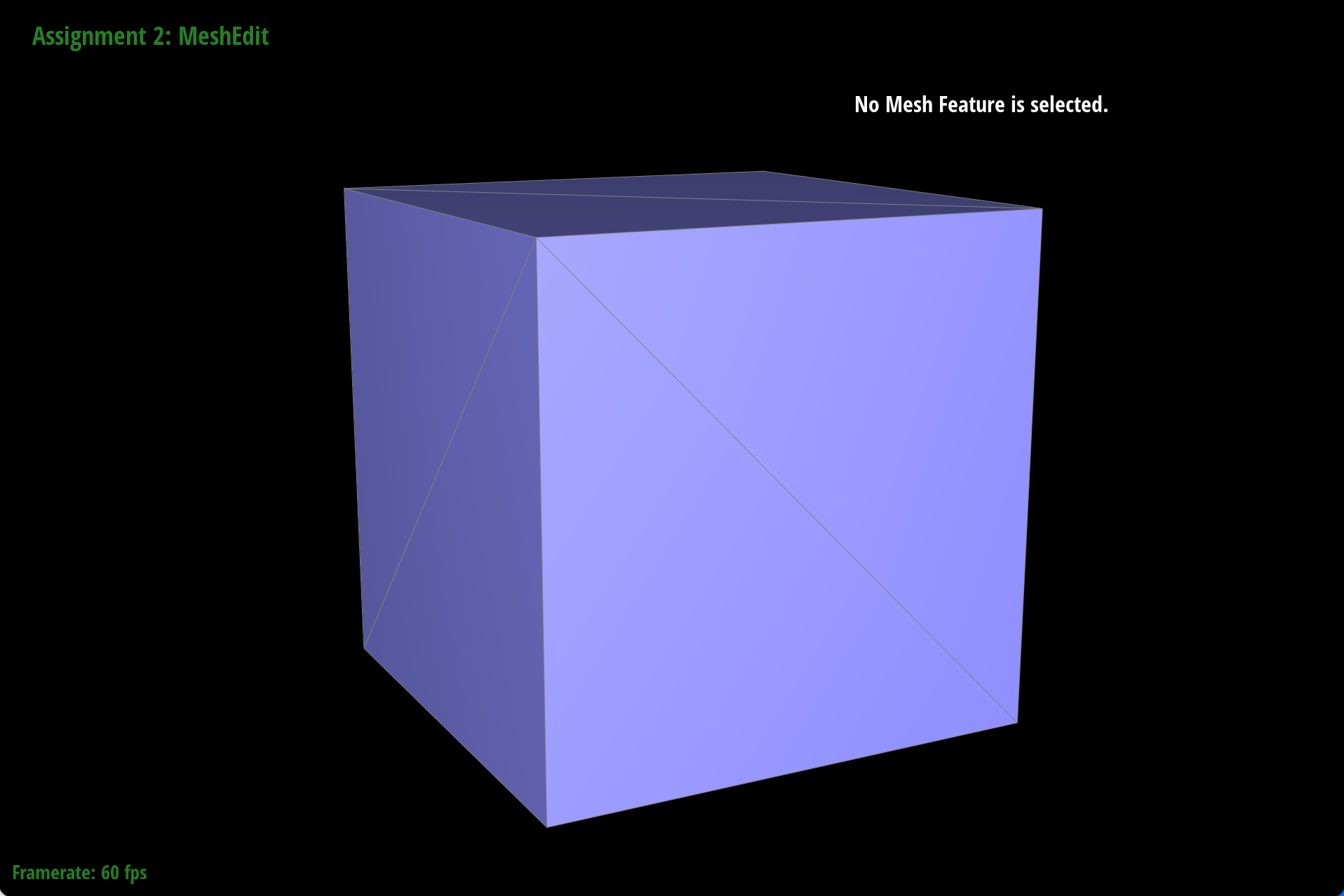
For example, notice how the pre-split cube has 4 triangular faces per square face, while the standard cube only has 2. The pre-split cube retains more of its shape as we upsample, while the standard cube becomes more asymmetric.