CS 184: Computer Graphics and Imaging, Spring 2023

Project 4: Cloth Simulator

Tyler Bhadra, Victor Zhang


Overview

In this project we implemented a cloth simulator using a grid structure of point masses and springs. We employed Verlet Integration and Hooke's Law to update the position of point masses, according to the forces acting upon them, and simulate the movement of cloth. In addition to the above, we also implemented a variety of GLSL shaders so as to give the cloth a more realistic appearance. This project gave us insight into the basic implementation framework of simulations. Namely, that many physical objects and phenomena (cloth, rope, soft and rigid bodies, water & fluid dynamics, etc...) can be modeled using a structure of point masses (or alternatively, particles) and springs, as well as the different force equations of the relative physical phenomena which can be used during numerical integration and position updates.

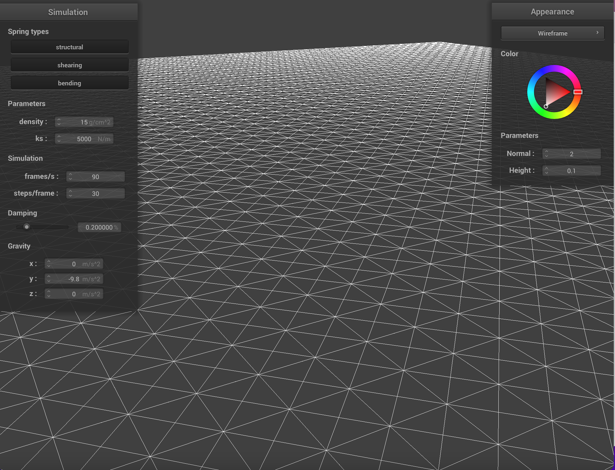
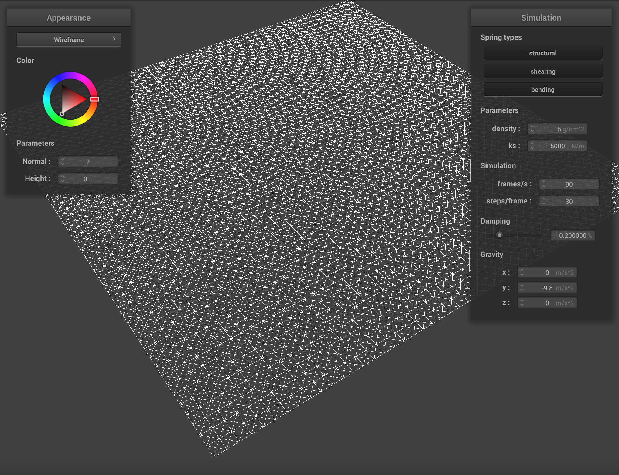
Part 1: Masses and springs

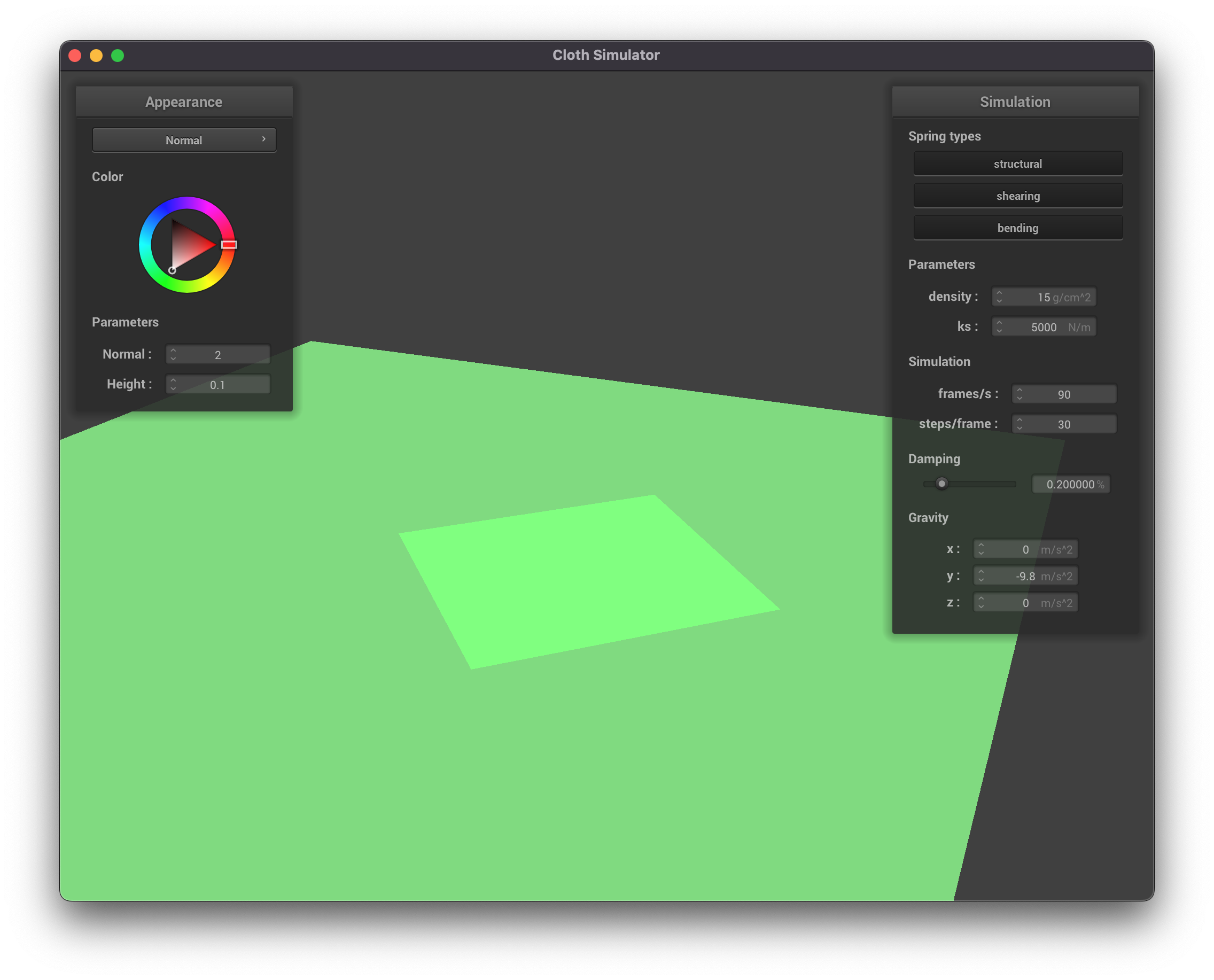
To model cloth we use a grid of point masses connnected by springs (Represented by the PointMass and Spring classes, respectively). More specifically, a Cloth object is initially defined by num_width_points x num_height_points uniformly spaced point masses placed within a horizontal or vertical width x height plane. These point masses are connected by three different types of springs, each representing a different constraint.

These three spring types represent (1) Structural Constraints, which exist between a point mass and the point mass to its left as well as the point mass above it, (2) Shearing Constraints, which exist between a point mass and the point mass to its diagonal upper left as well as the point mass to its diagonal upper right, and (3) Bending Constraints, which exist between a point mass and the point mass two away to its left as well as the point mass two above it.

Closeup of the point mass grid structure
With all contraints
With only shearing constraint
Without shearing constraints

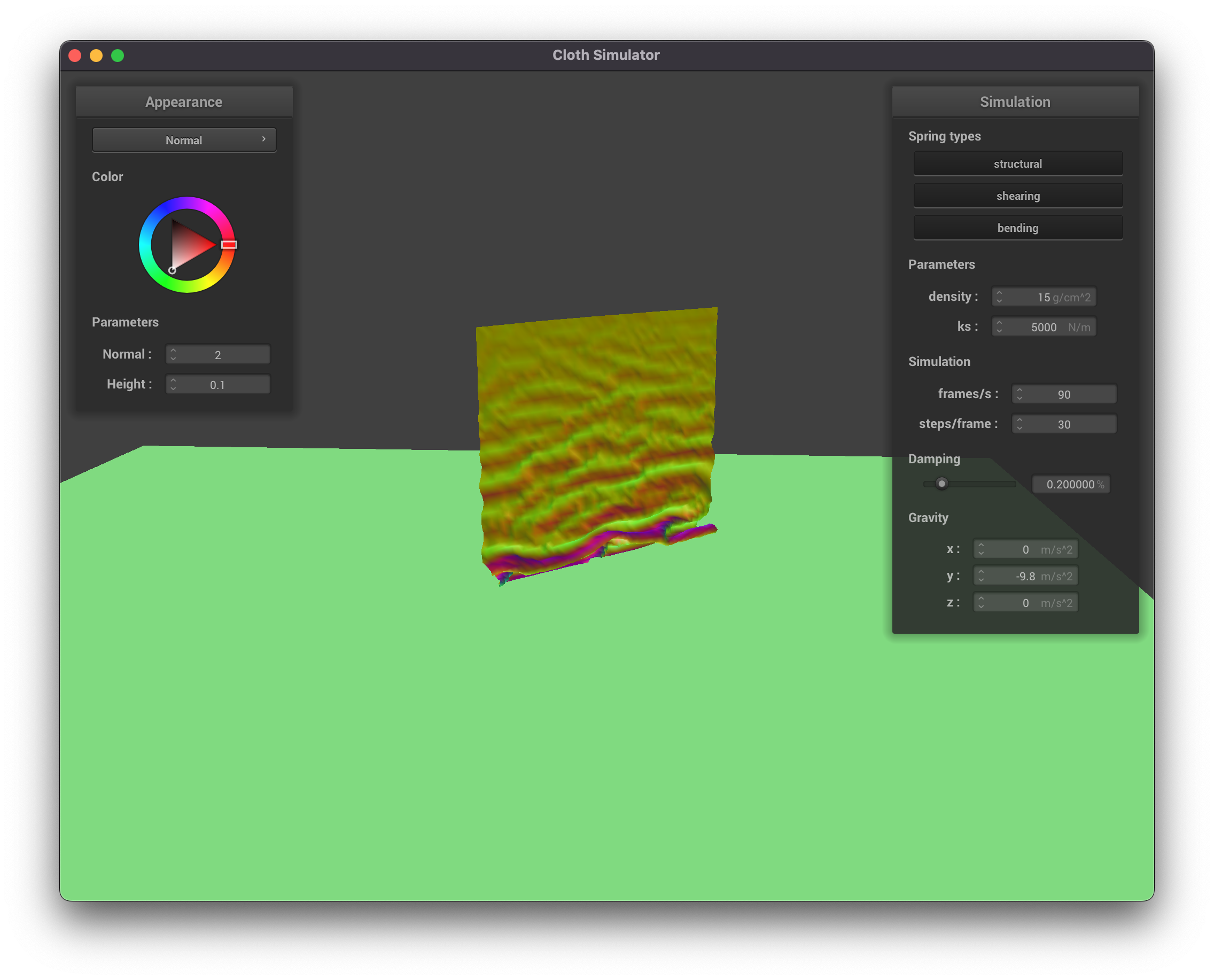
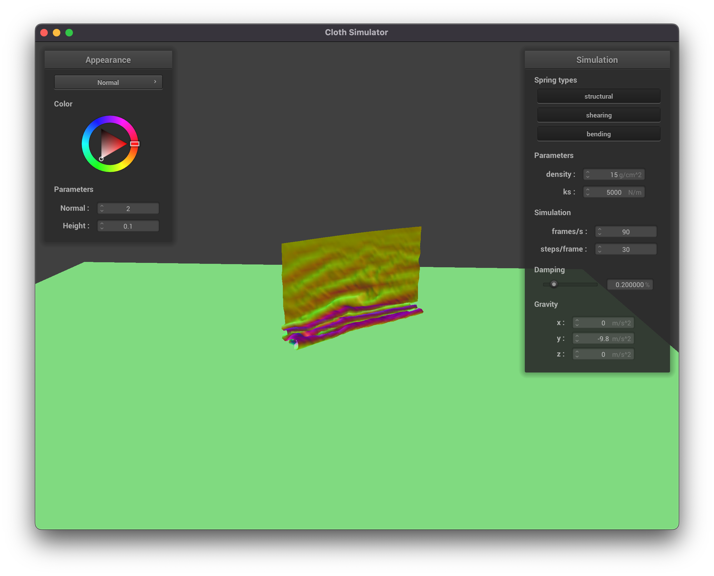
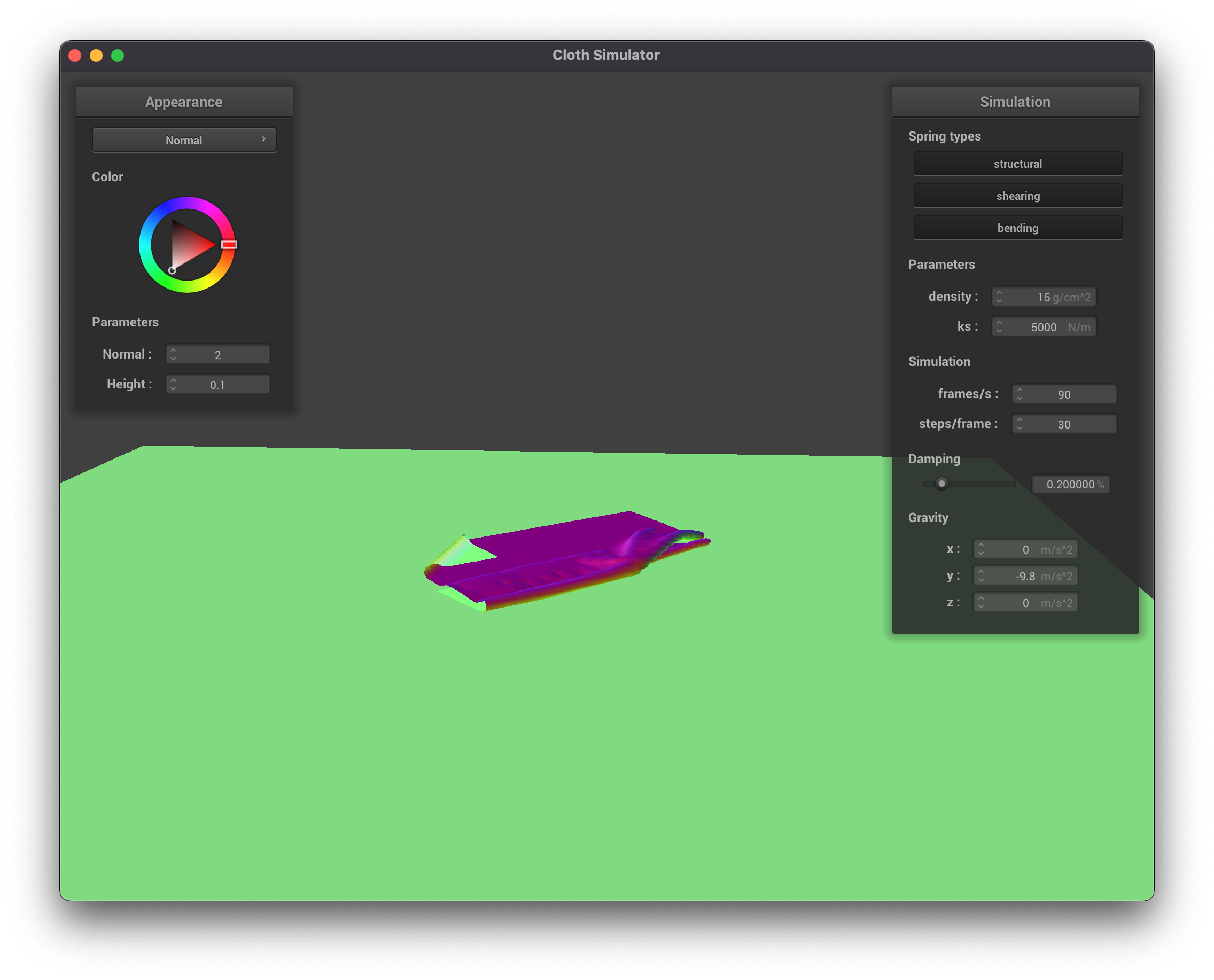
Part 2: Simulation via Numerical Integration

In order to simulate the movement of cloth, we compute the total forces acting on each point mass (external forces + the spring forces, derived from Hooke's Law) then use Verlet Integration to calculate the next position of each point mass.

During the computation of forces we first accumulate force values (per point mass p) from all external forces acting on p, such as gravity, using Newton's 2nd law F = ma. Once external forces have been accumulated we calculate all spring forces Fs acting on the point masses pa and pb of every spring using Hooke's Law ( Fs = ks * (||pa - pb|| - l )).

After the accumulation of forces, we use Verlet Integration to calculate the new position at time t + dt, xt+dt as follows:

xt+dt = xt + vt * dt + at * dt 2

We estimate vt * dt as xt - xt-dt and apply a damping term 1 - d such that our equation becomes:

xt+dt = xt + (1 - d ) * (xt - xt-dt ) + at * dt 2

Where at equals the forces acting on the p at time t divided by the mass of p.

To ensure that springs are not unreasonably deformed during each timestep, we constrain the computed position updates using the method outlined in section 5 of the SIGGRAPH 1995 Provot paper on deformation constraints in mass-spring models. With a critical deformation rate of 0.1 we can correct the positions of two point masses such that the spring's length is at most 10% greater than it's rest_length at the end of any time step t.

Default parameters

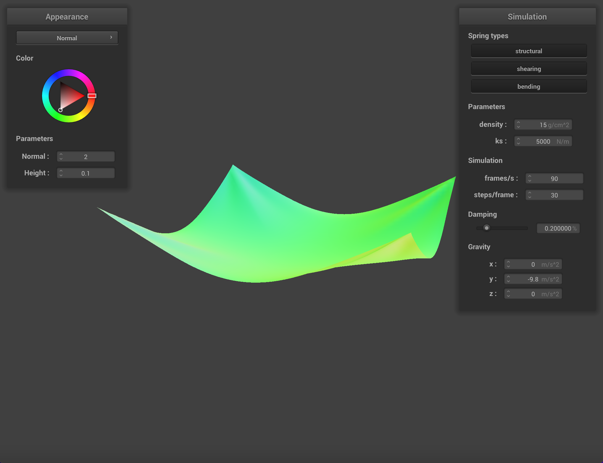
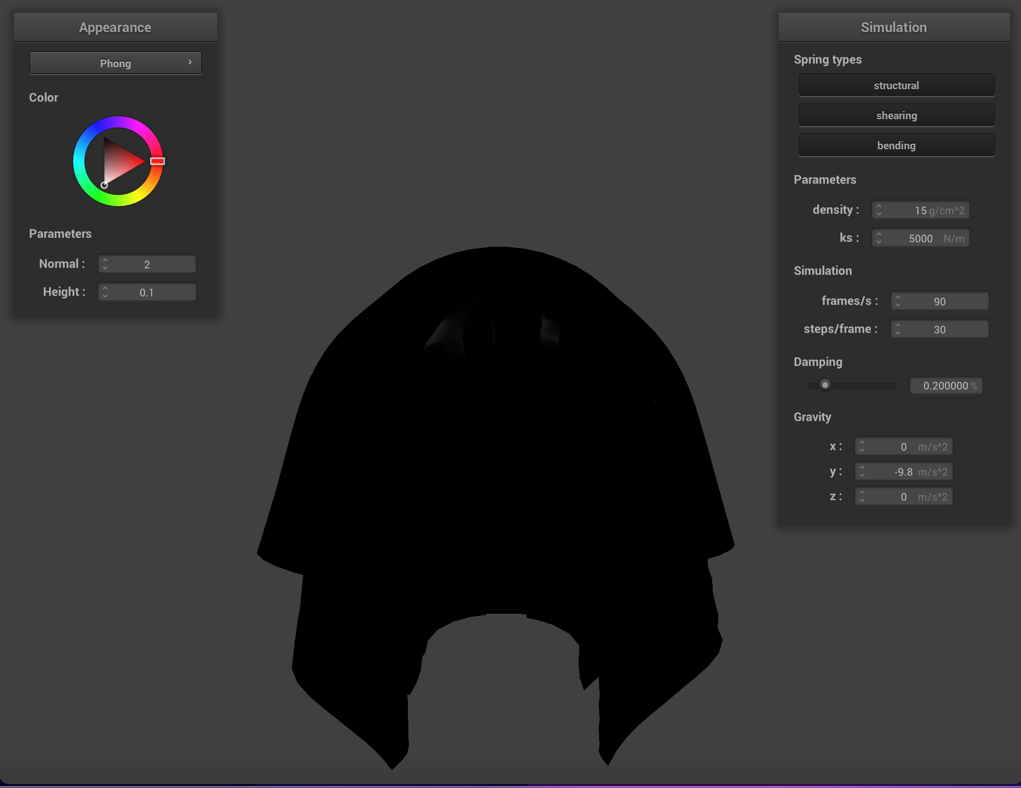
Below are images of two pieces of cloth (each with 2 pins) with different ks values at rest. The spring constant ks represents the "springyness" of our springs. The larger the ks, the stiffer our cloth is. With a ks of 50 N/m the cloth generally has a looser, wrinkly look, whereas a ks of 50000 N/m yields a cloth with a more taut appearence.

ks = 50 N/m
ks = 50000 N/m

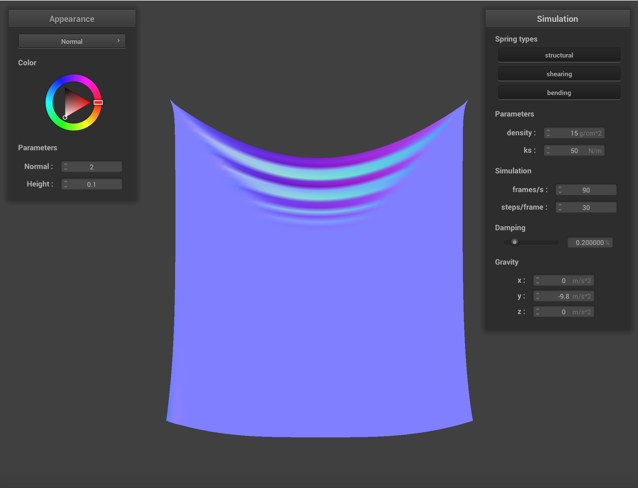
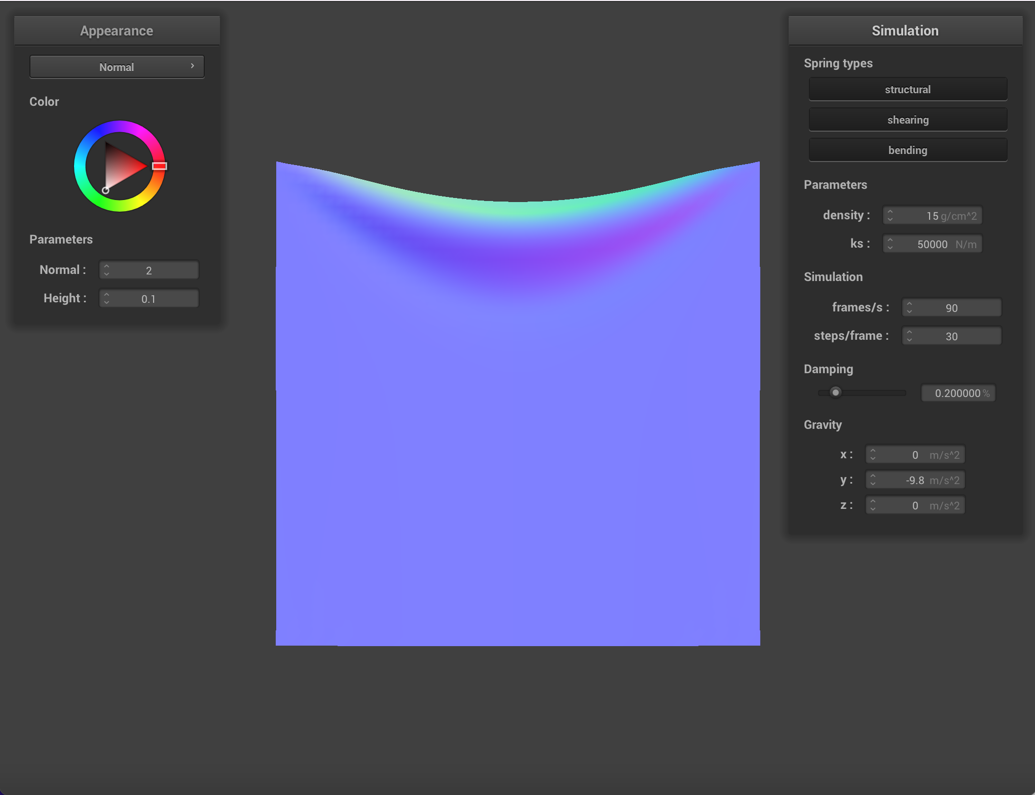
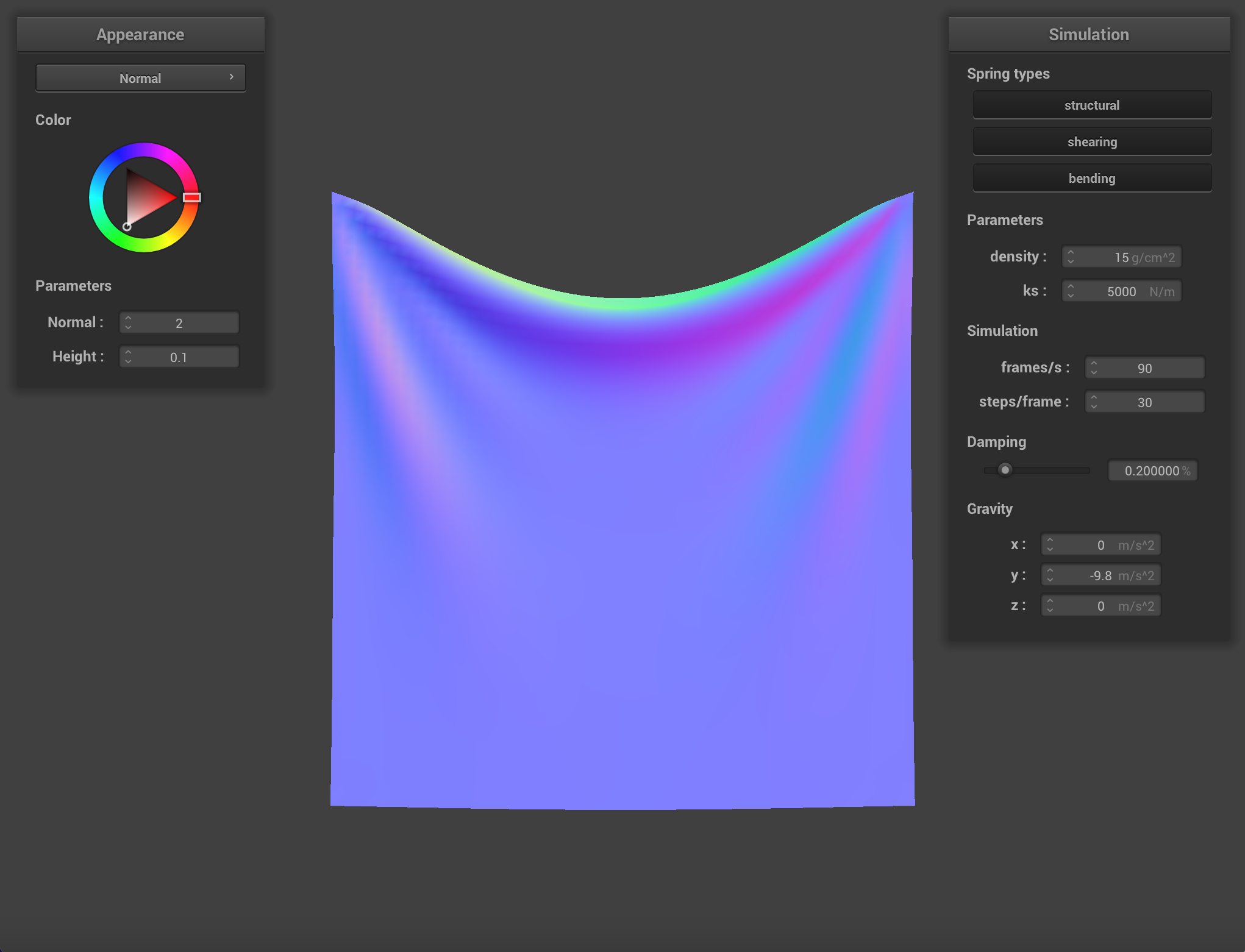
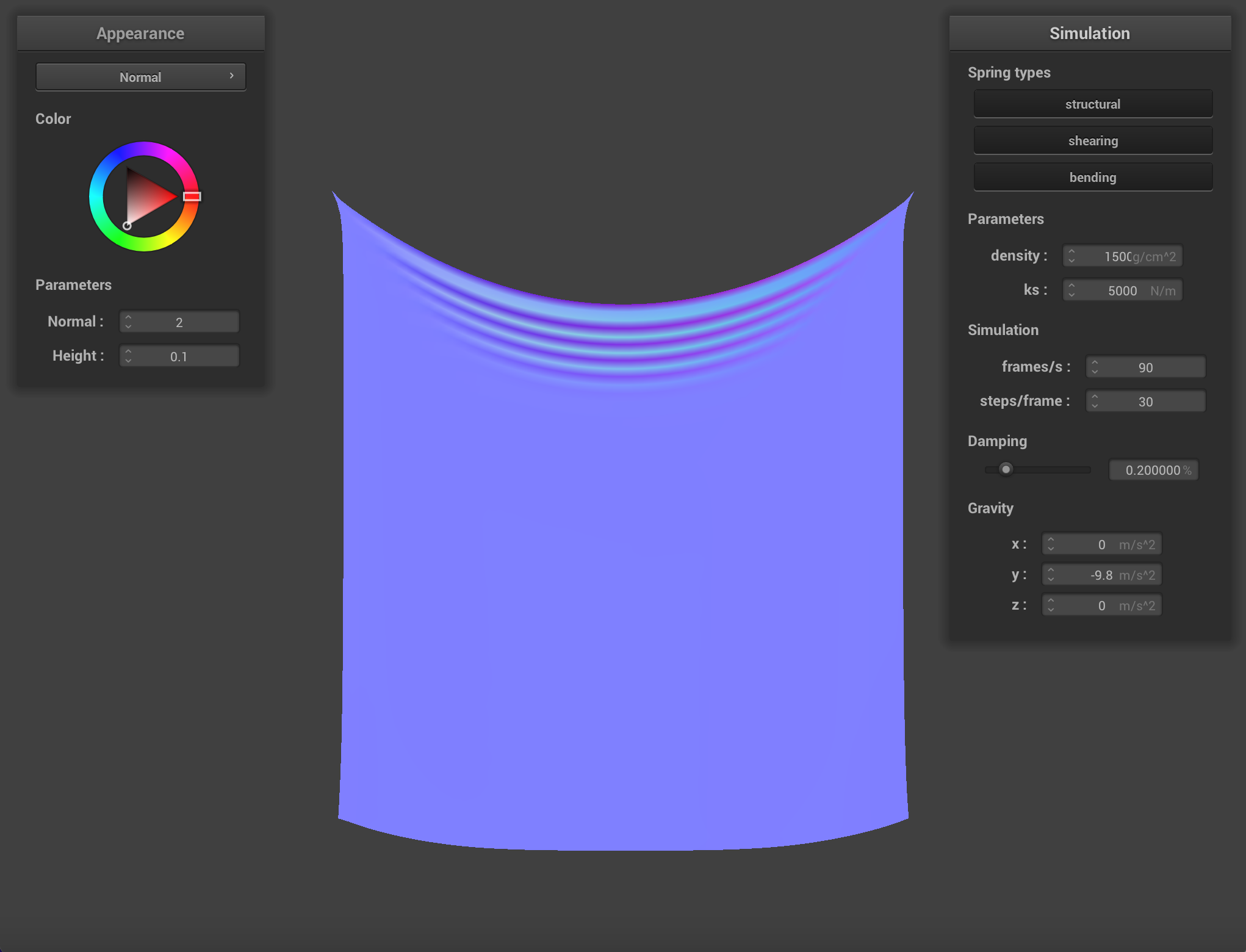
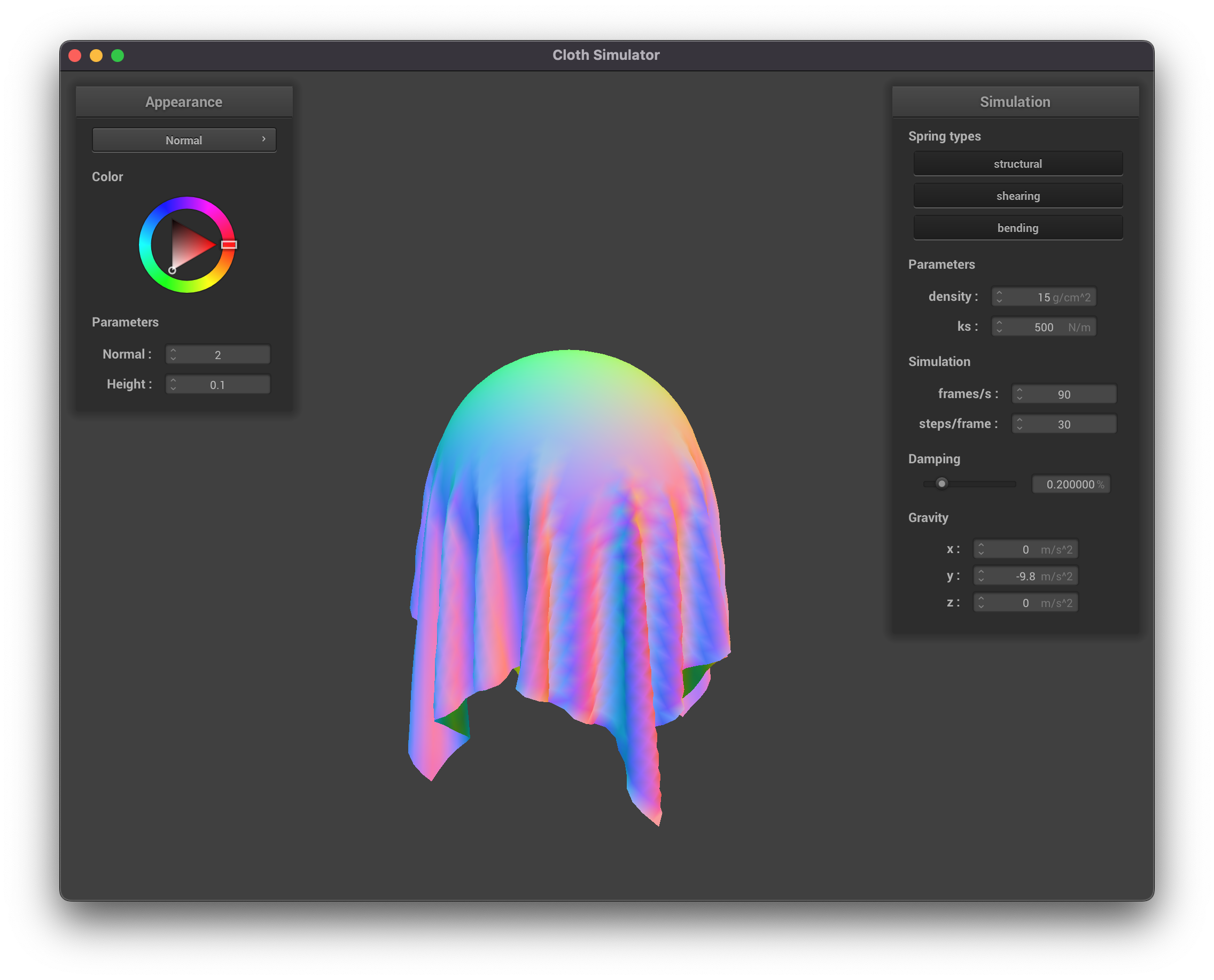
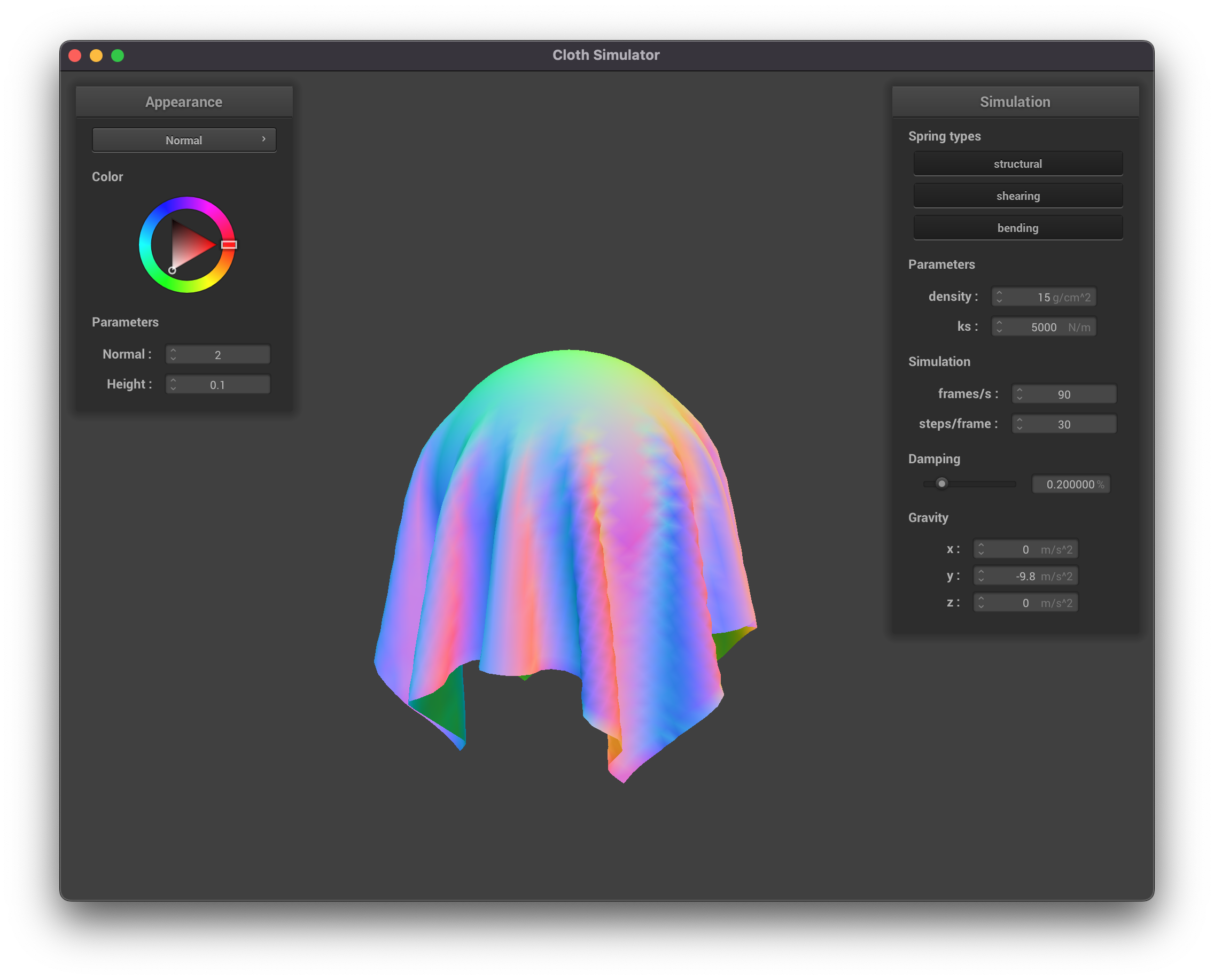
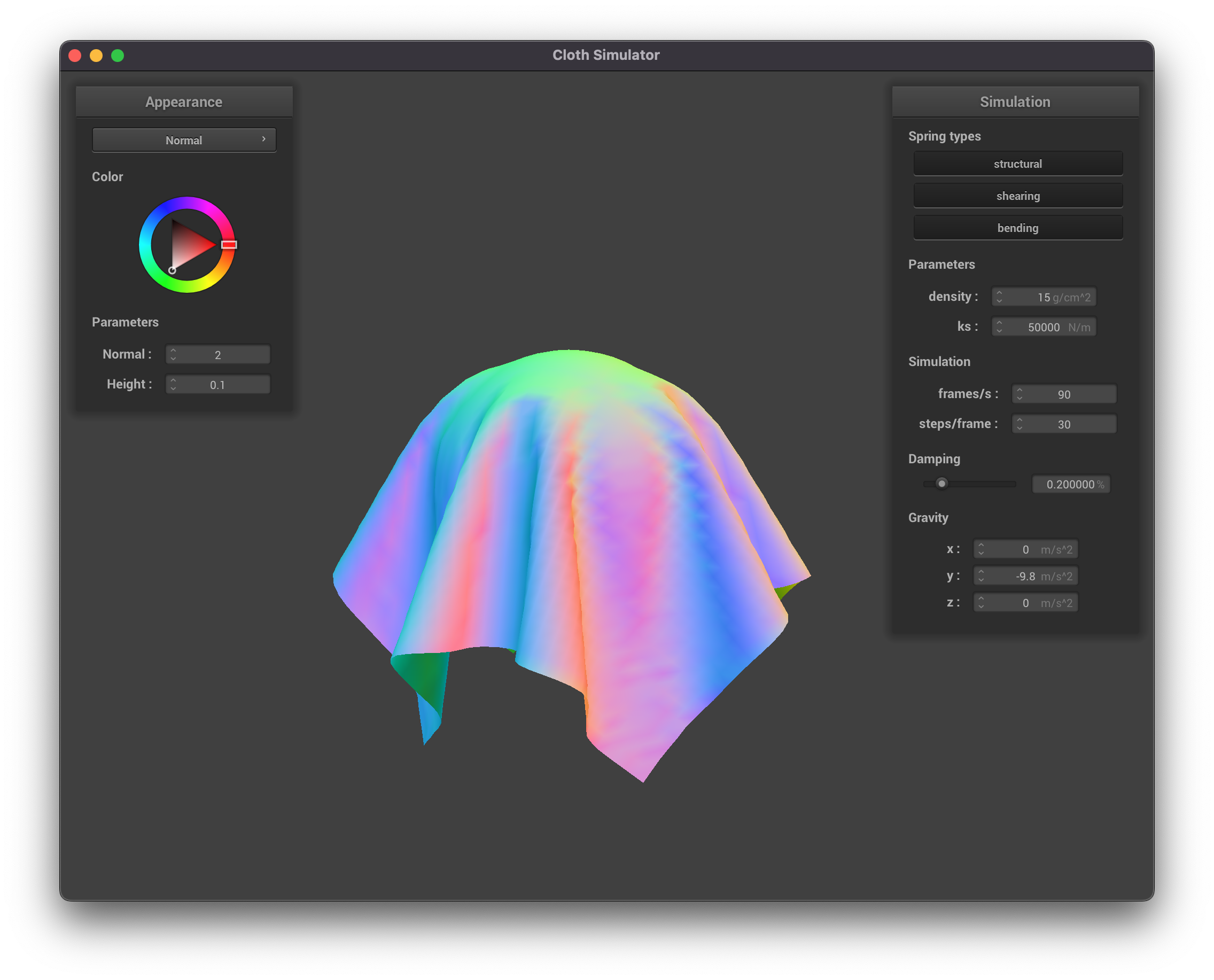
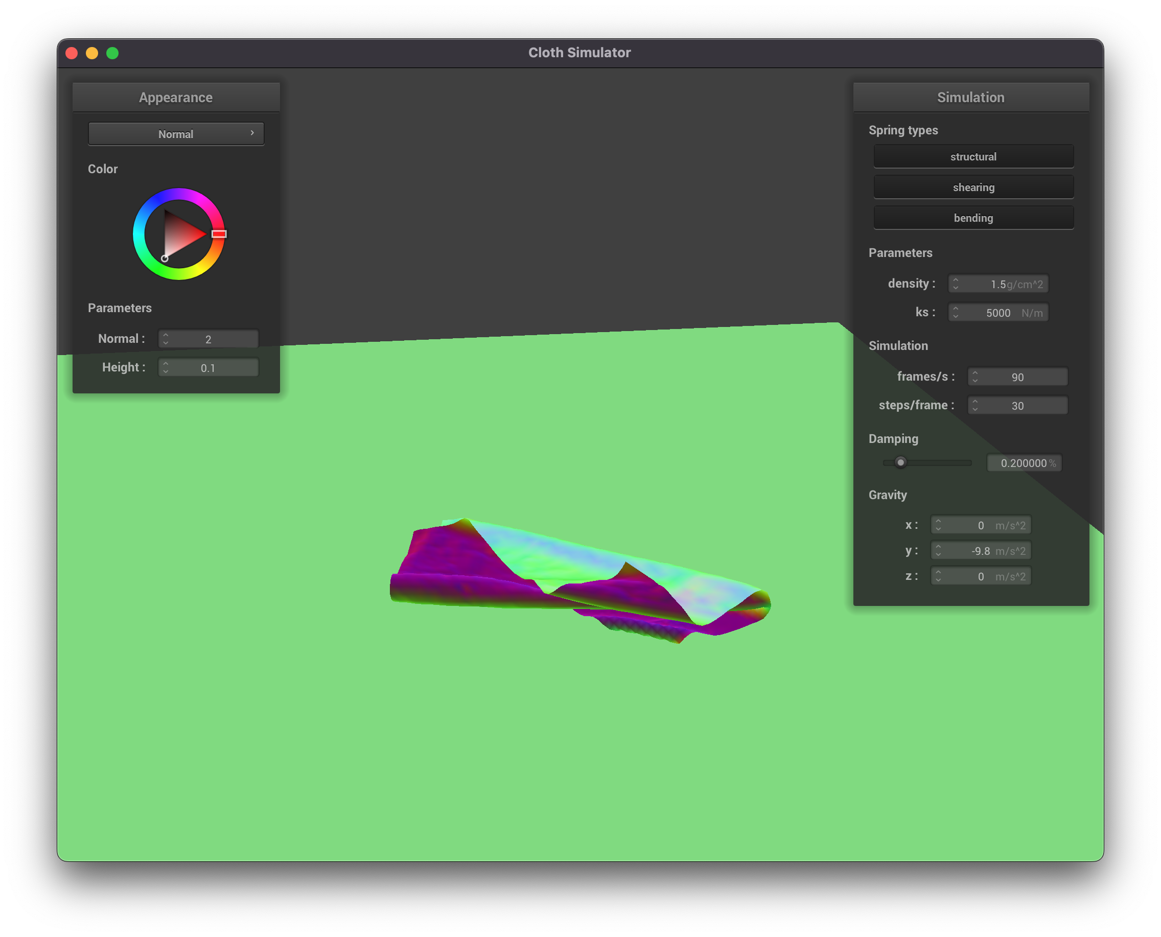
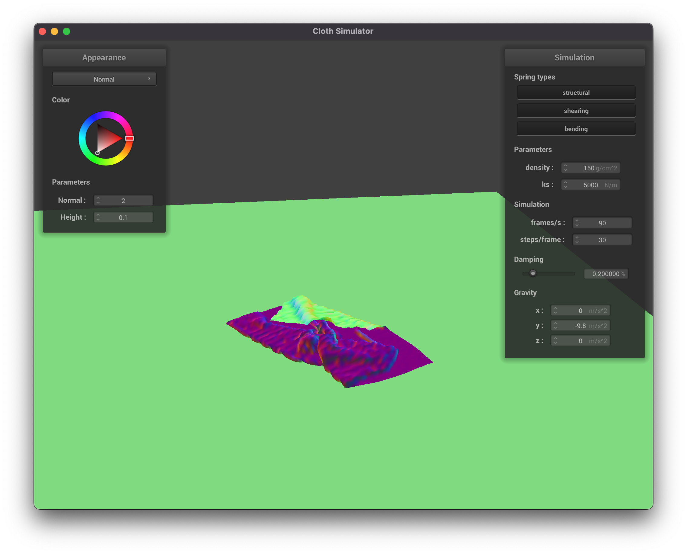
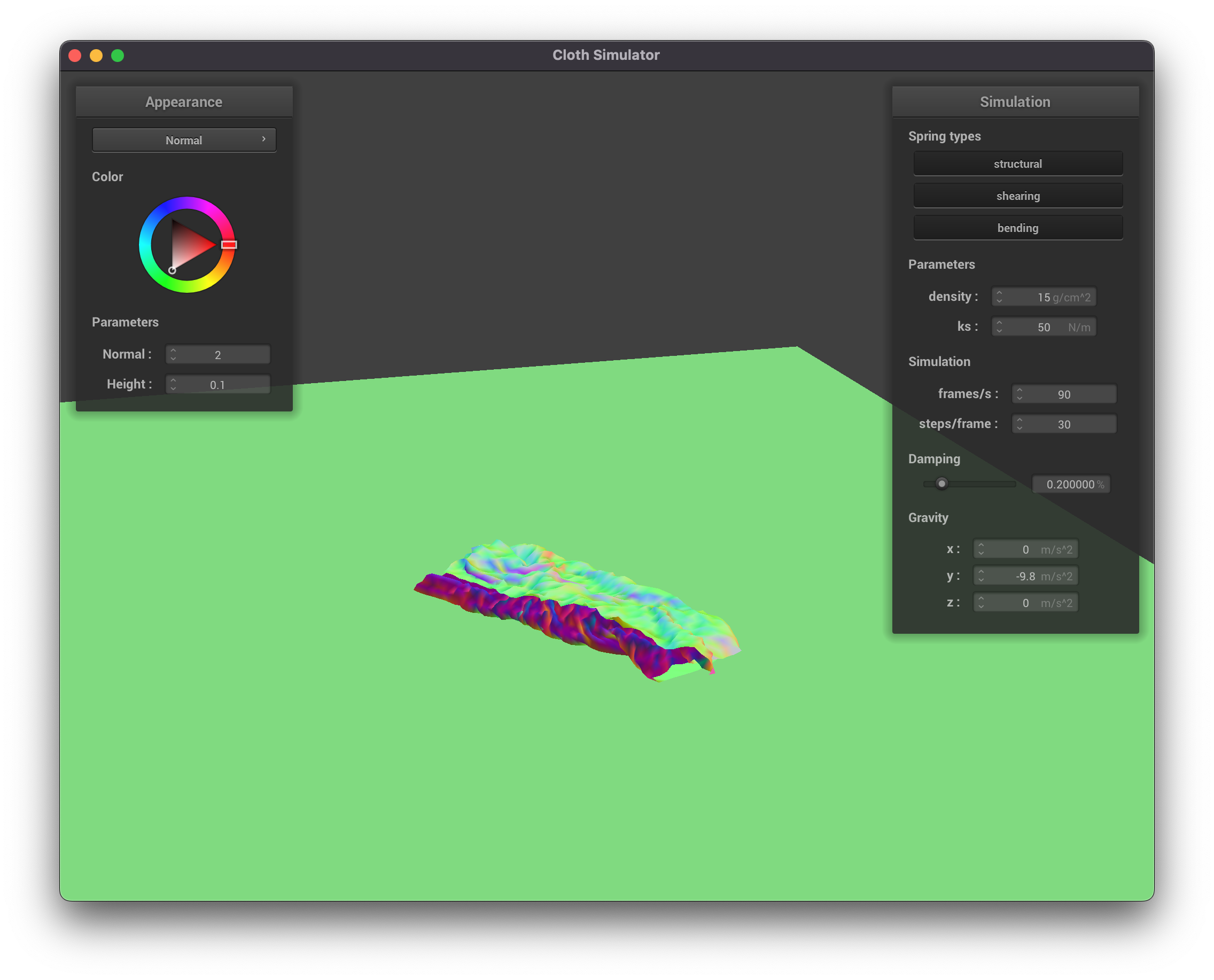
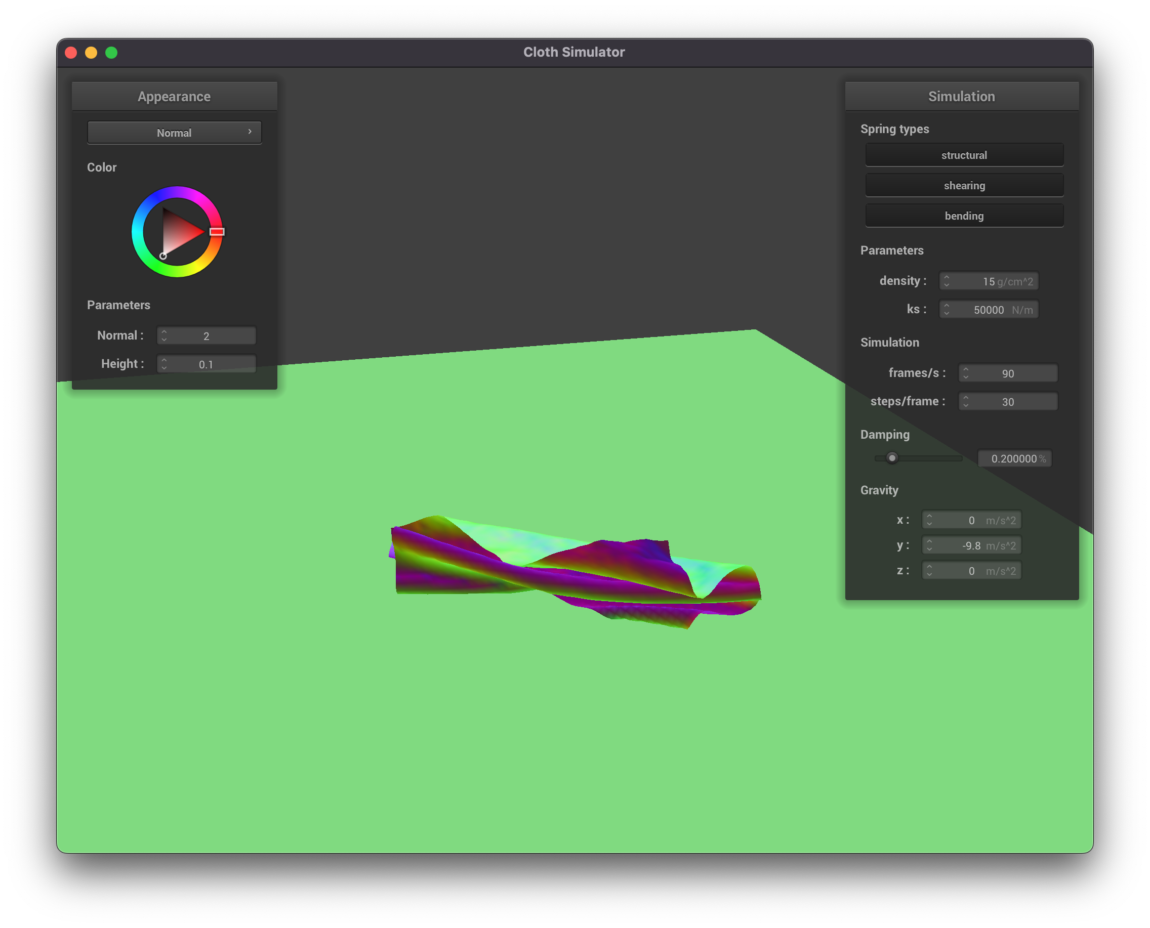
Density affects how heavy the cloth appears to be. A cloth with a density of 15 g/cm2 appears lighter than a cloth with a density of 15000 g/cm2, which has many thin, closely occuring folds indicating a greater perceived heaviness.

density = 15 g/cm2
density = 15000 g/cm2

Damping affects how fast the energy in the system decays. In this case, the most obvious visual indication of this energy is how much the cloth swings. With a damping value of 0.0%, the cloth swings wildly and unrealistically, never coming to a stable rest position. With a damping value of 1.0%, the cloth falls very slowly and comes to rest with almost no apparent extra movement (For example, with default parameters the cloth swings back and forth very slightly before coming to rest).

damping = 0.0%
damping = 1.0%


Cloth with 4 pins, at rest, using normal shading.

Part 3: Handling Collisions with Other Objects

ks = 500
ks = 5000
ks = 50000
When we look at the different images, it seems that as the ks value increases, the cloth seems stiffer since it hangs less limply off the sphere and instead the cloth increasingly hangs off at an angle, as if something is supporting the cloth.
Cloth resting on the plane


Part 4: Handling Self-Collisions
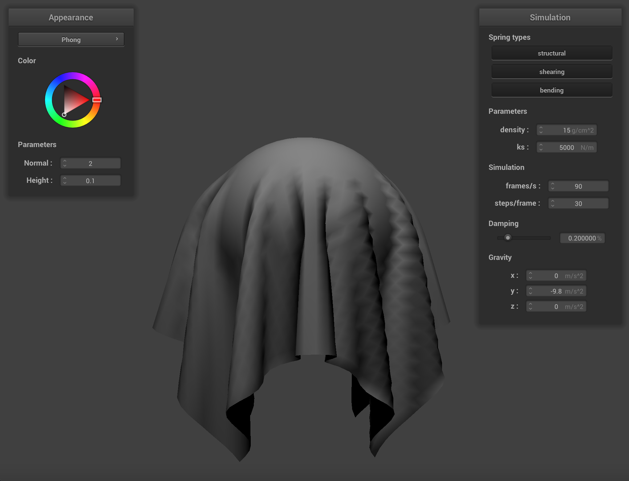
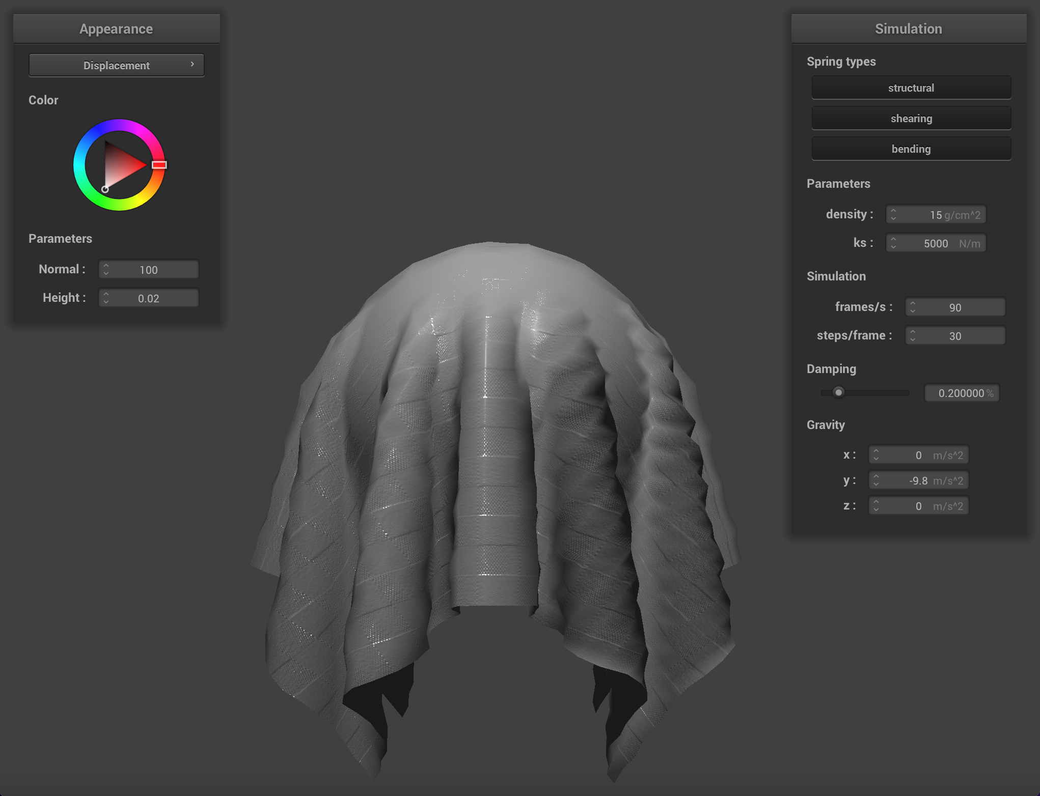
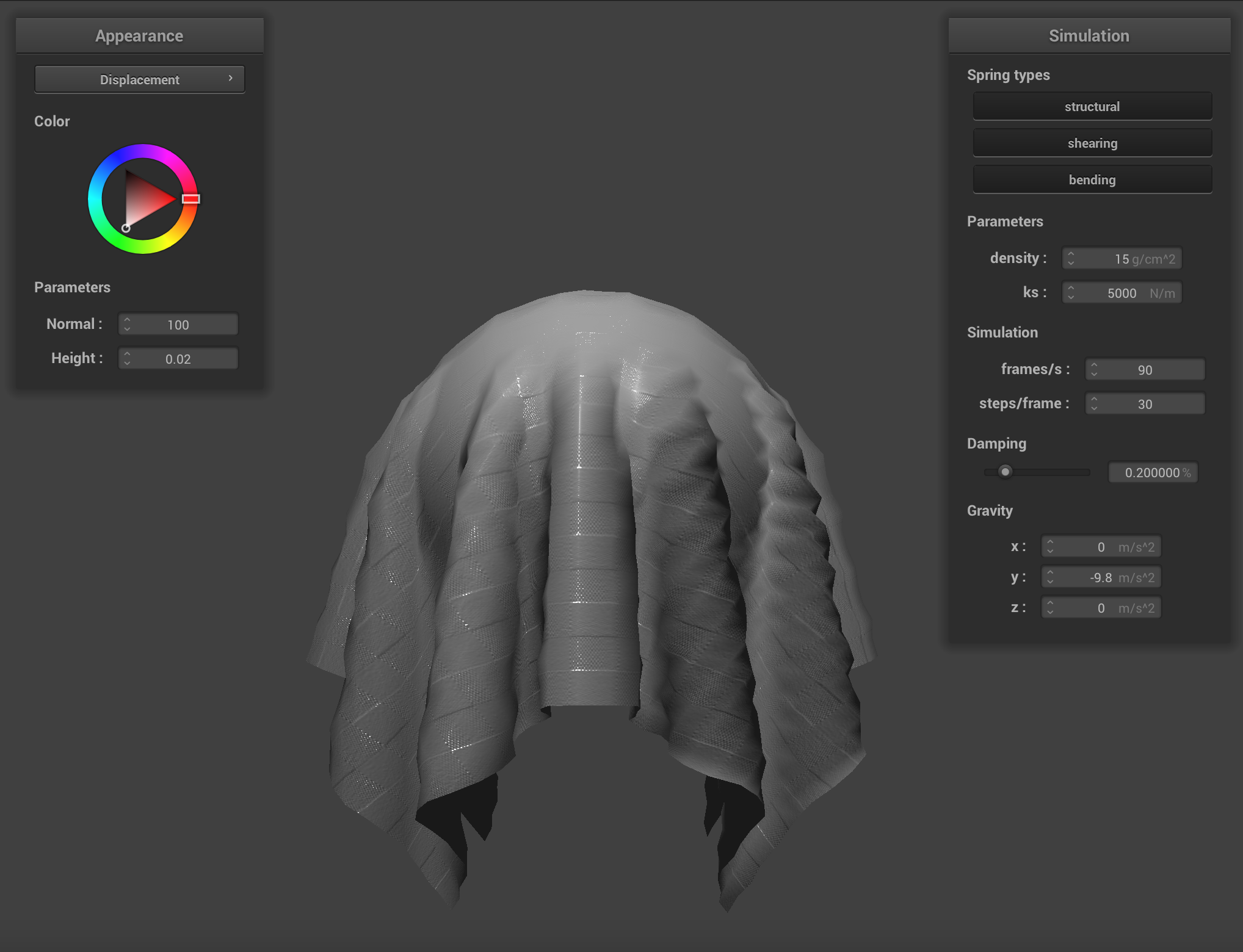
Start of the self-collision
Midway through the self-collision
Resting state
Low density
High Density
Low ks value
High ks value
It looks like low density and a high ks value both have similar effects on the cloth during self collision. The same can be said about high density and a low ks value. In the low density/high ks value case, the cloth seems stiffer, as if it were actually made of rubber. It has less creases and instead tends to be flatter with smooth, uninterrupted curves. In the high density/low ks value case,


Part 5: Shaders

At this point our cloth behaves in a realistic manner, but because its rendered with basic normal shading it doesn't look like it's made out of realistic material. Using a computation heavy raytracing algorithm on the CPU to render every frame of a real time simulation would be extremely slow. Therefore, in order to achieve similar results, we implemented a couple GLSL shader programs that allowed us to render realistic material quickly. This is because shaders are isolated programs that run in parallel on the GPU, handling parts of the graphics pipeline. They take in information such as lighting computation values, color parameters, texture files and vertex attributes, and output a single four-dimensional vector storing information about vertex positions and color values.

In GLSL there are two basic types of shaders. Namely, vertex shaders and fragment shaders. Vertex shaders apply transformations to vertices, storing the final position of a particular vertex in gl_Position and writing other relevant vertex information into varying constructs, which act as a sort of buffer or variable in which data (transformed vertex positions, normals, uv coordinates) can be passed on to a fragment shader for future use. Fragment shaders generally take in geometric attributes, such as the vertex position and normals that are calculated by a vertex shader, and use them to compute a color value to write to out_color.

One of these shaders uses the Blinn-Phong shading model which calculates the total reflected light as the sum of reflected ambient light (La), reflected diffuse light (Ld), and reflected specular light (Ls) as follows:

L = La + Ld + Ls

Or, in its expanded form:

L = kaIa + kd (I / r 2) max(0, n • l) + ks (I / r 2) max(0, n • h) p

In this equation the vector normal n, light intensity I, camera position, and light position are uniforms passed into the shader which we can use to calculate the light direction r, the normalized light direction vector l, the normalized view direction vector v, and the normalized half vector h calculated as the sum of v and l. The ambient coefficient ka, diffuse coefficient kd, specular coefficient ks, ambient light intensity Ia, and specular hardness exponent p, are all arbitrarily defined in the shader program (values were chosen as such to achieve the most subjectively realistic appearance: ka = 0.1, kd = 0.8, ks = 0.5, Ia = <1, 1, 1>, p = 100).


Ambient component only

Diffuse component only

Specular component only

All components

Texture mapping shader using a pixellated image from the Magic the Gathering card Dreamroot Cascade


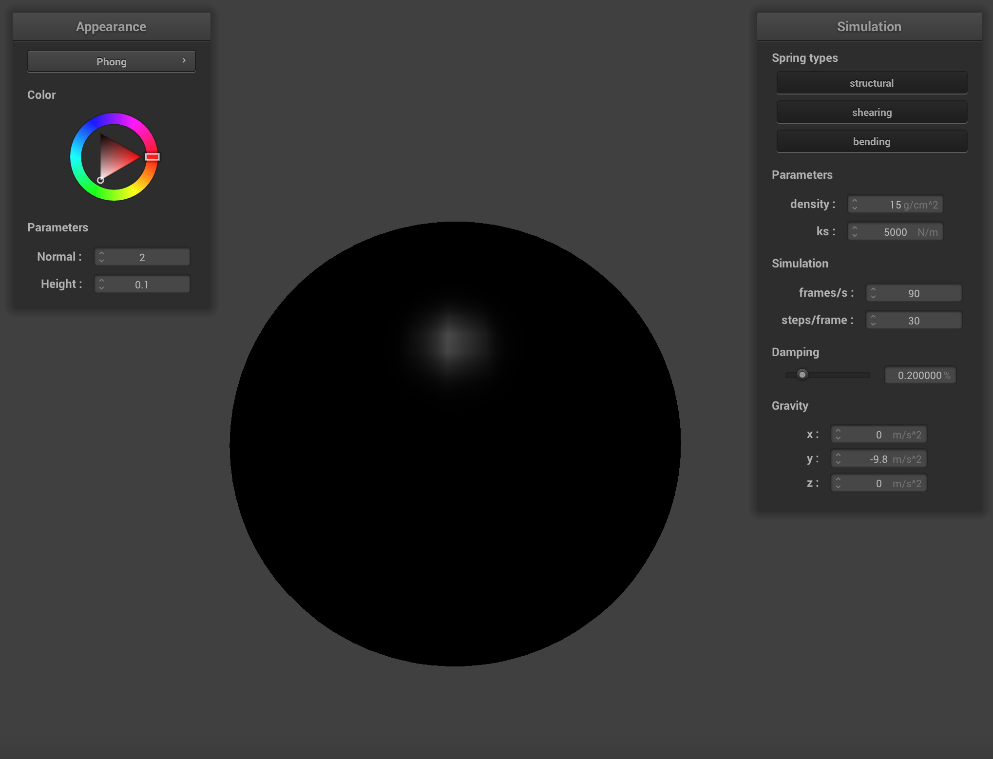
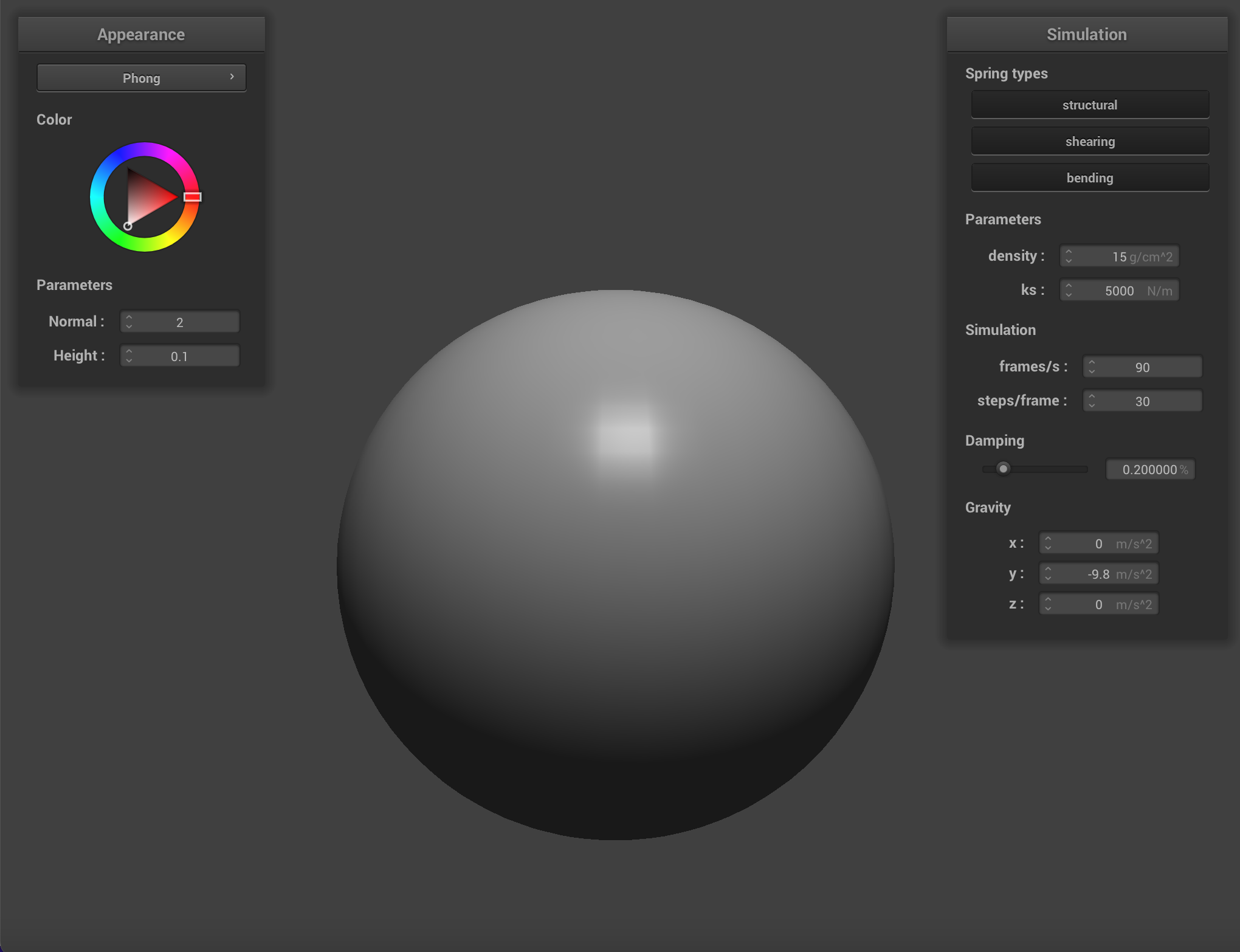
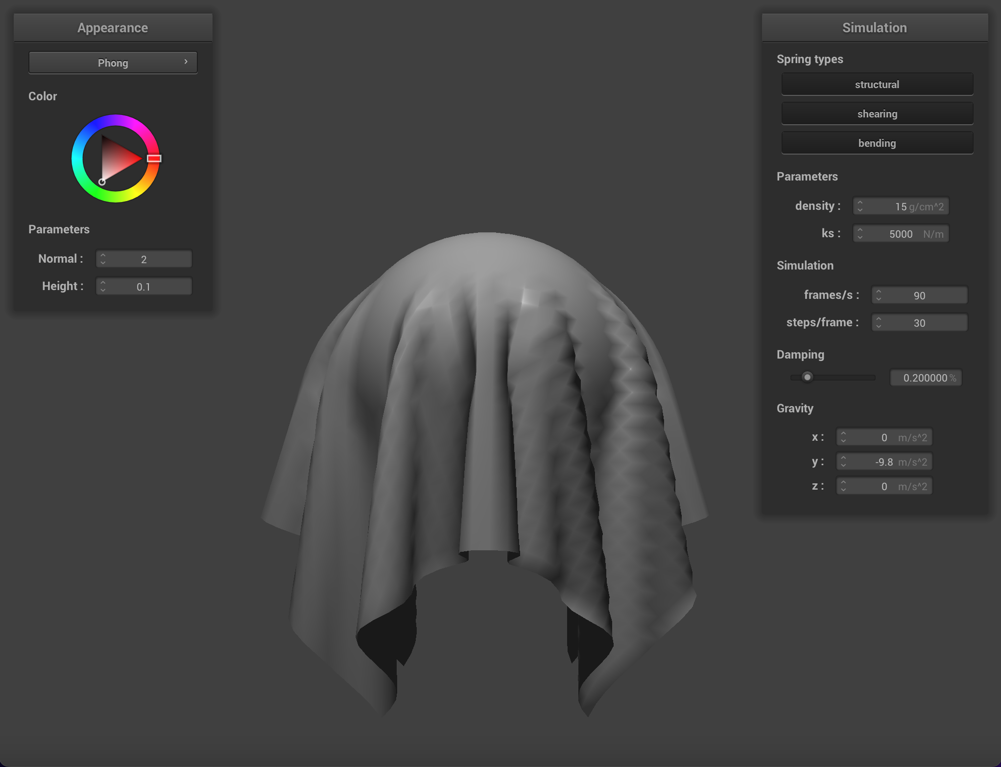
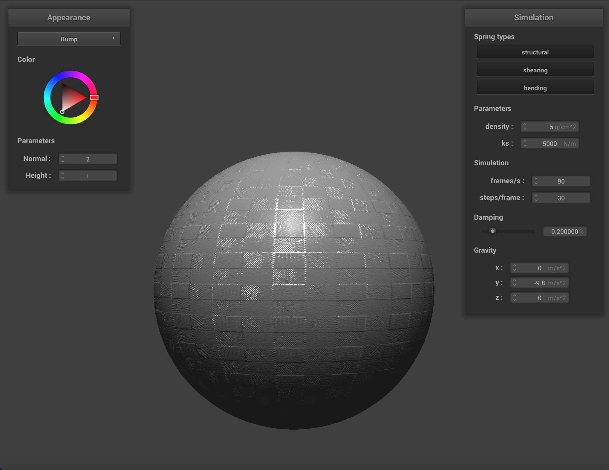
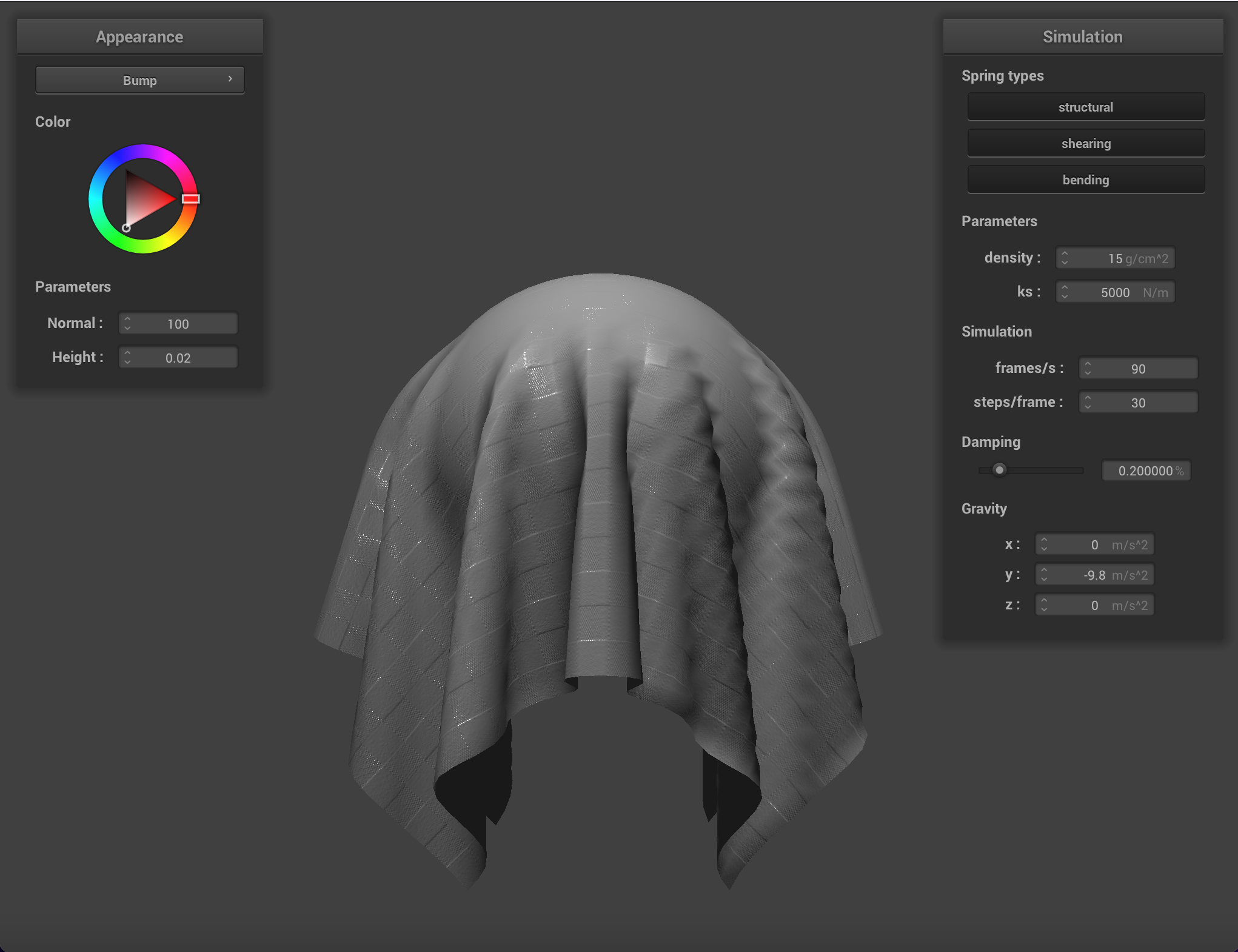
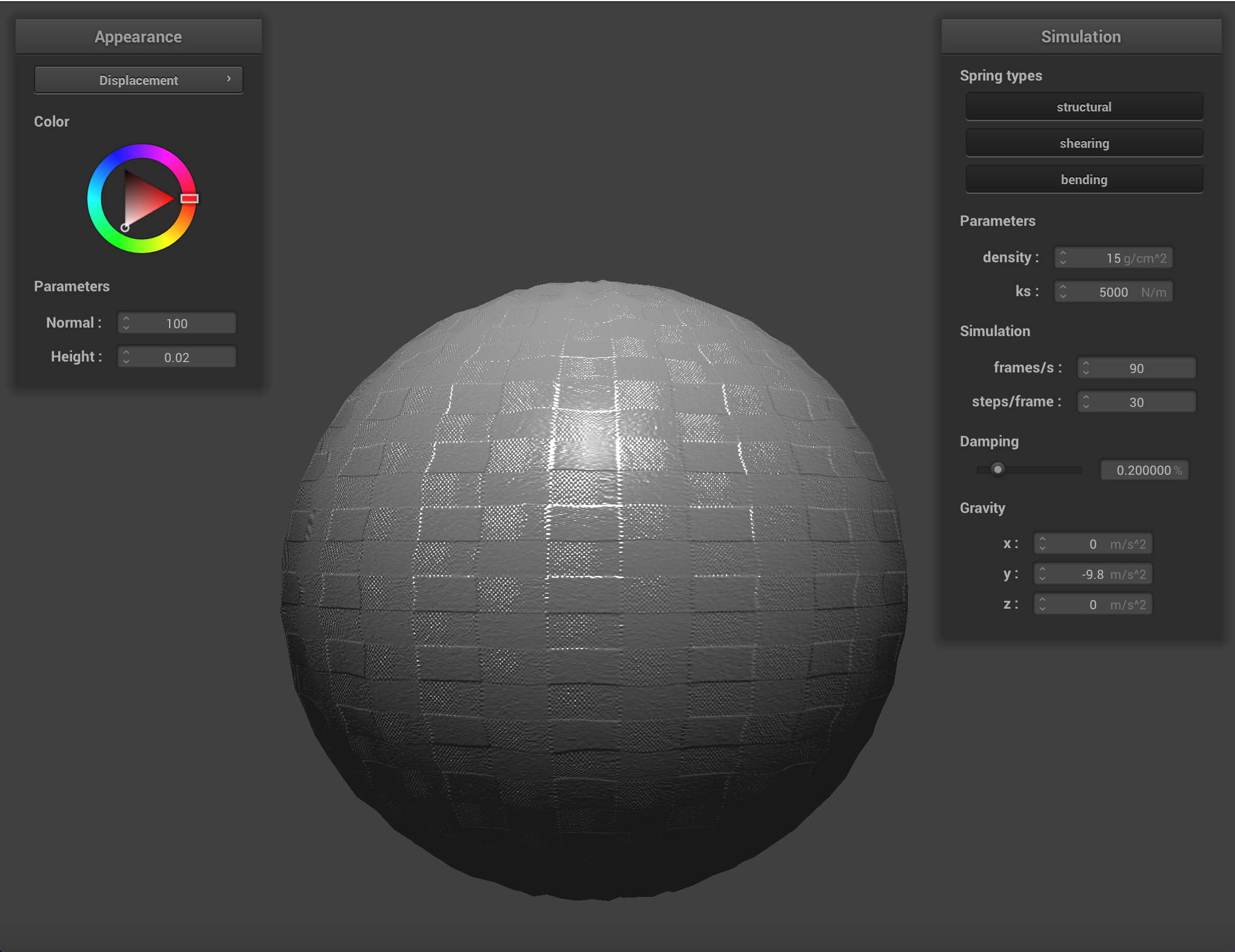
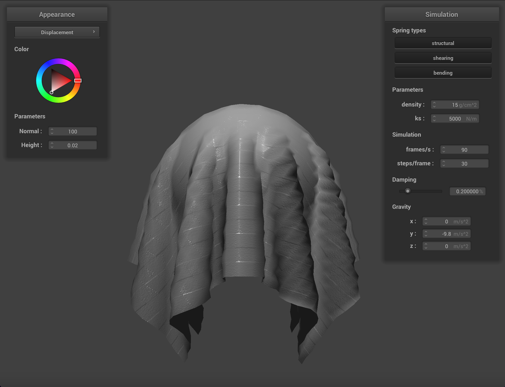
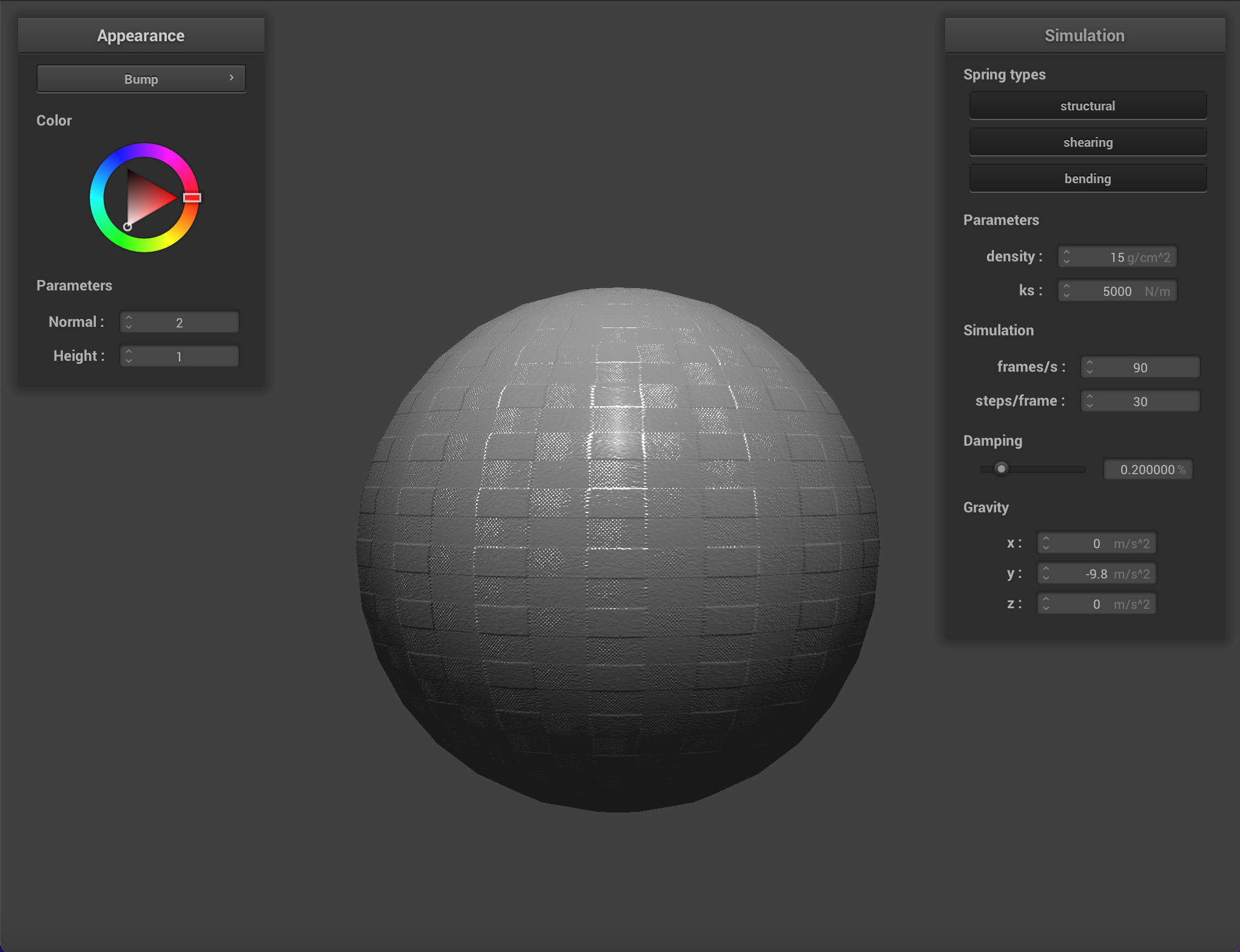
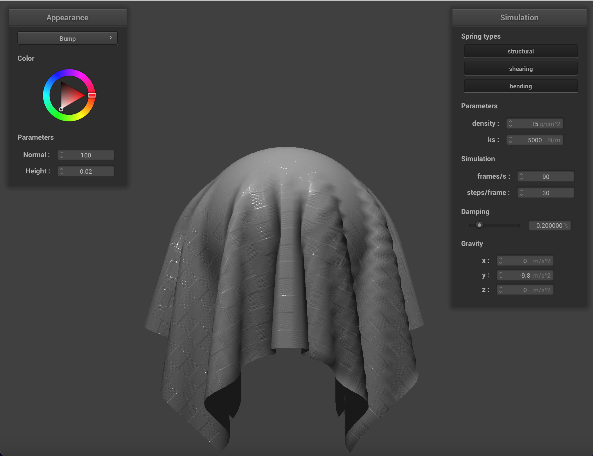
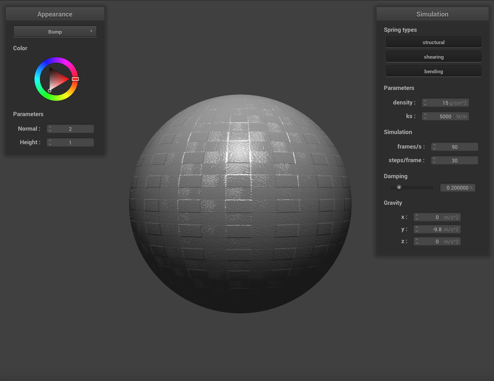
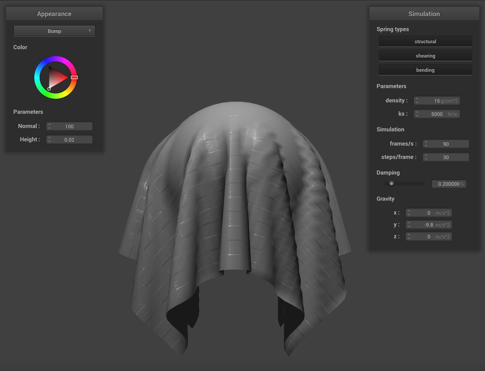
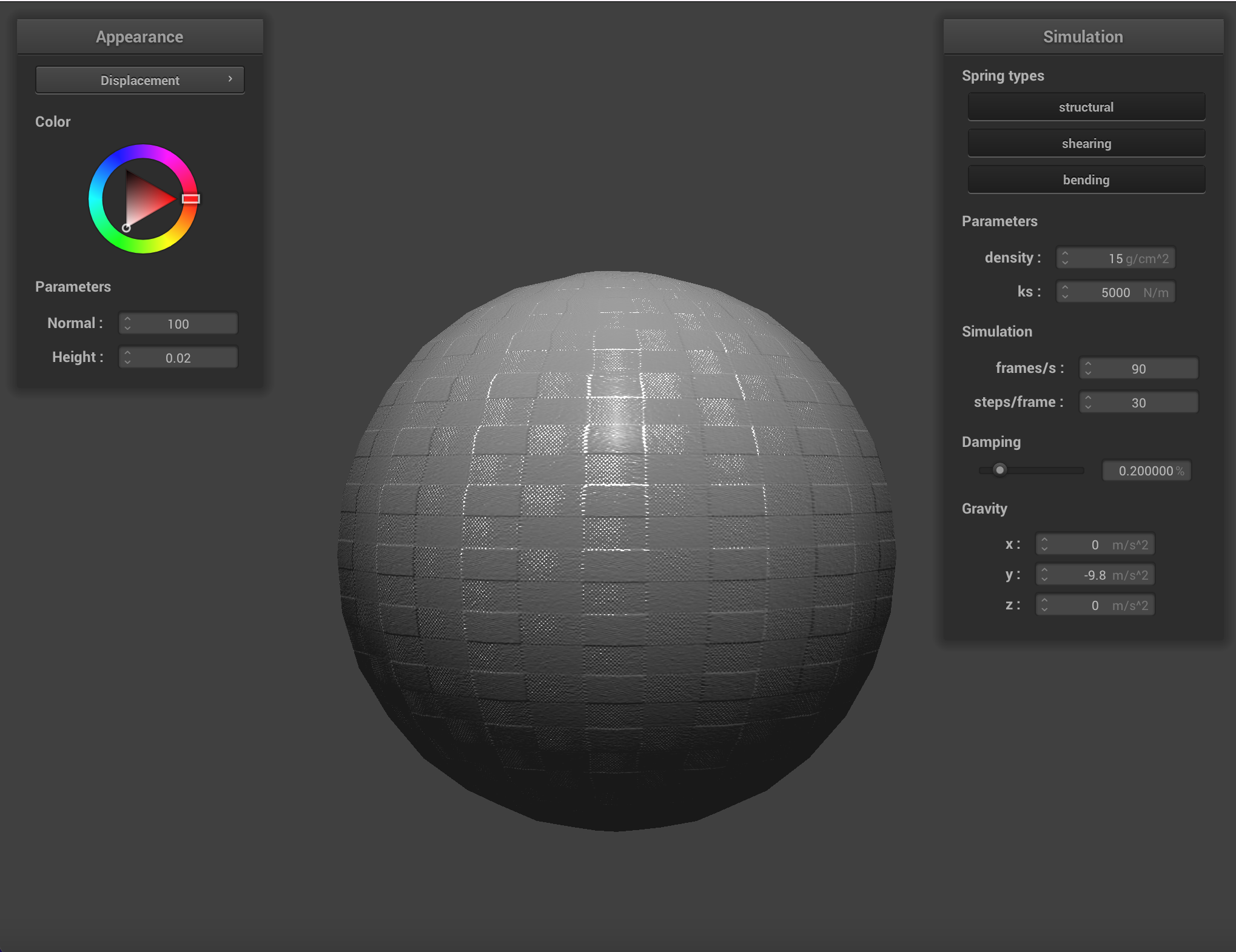
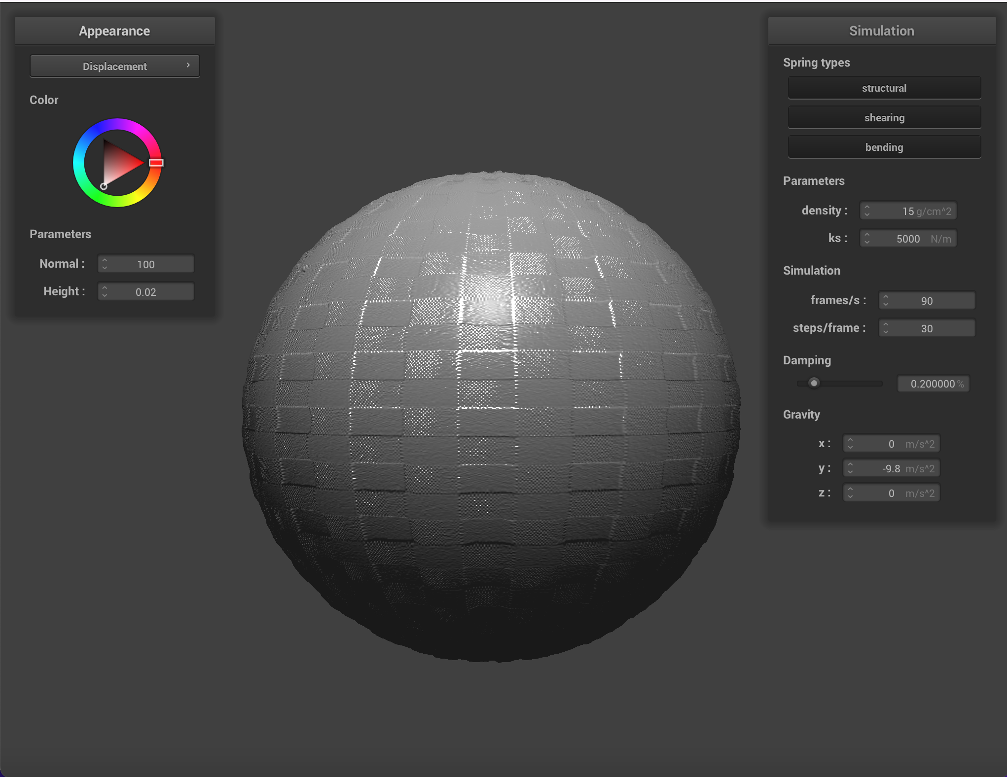
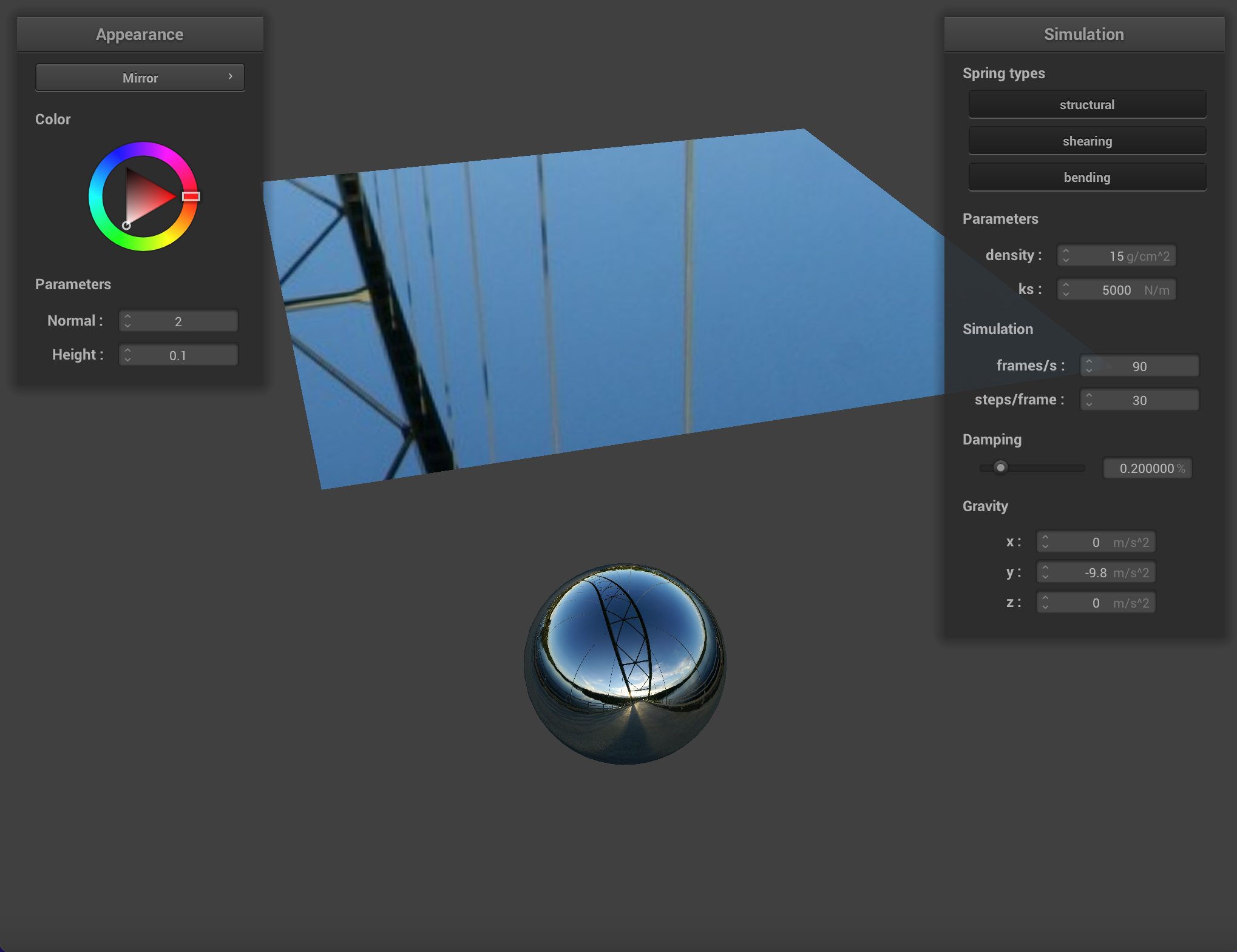
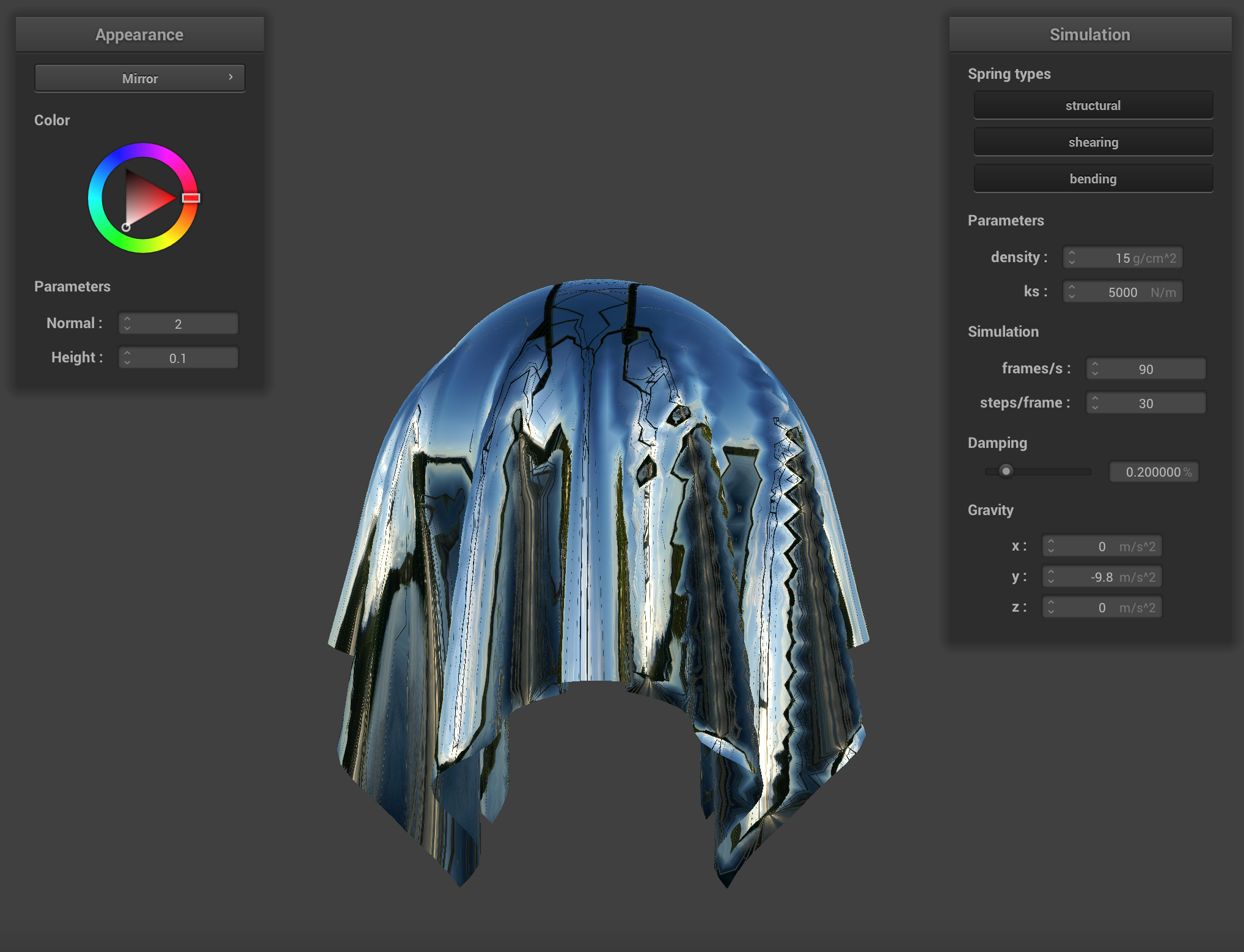
We can apply finer detail (or at least the illusion of finer detail) to texture mappings by implementing bump mapping and displacement mapping, which allow a shader to process a height map encoded in a texture and apply it to the final out_color value. In bump mapping we modify the normals of an object in the fragment shader, using the modified value in our lighting calculations so as to give the illusion of fine detail (such as bumps and grooves) on the texture. In actuality, the topography of the texture mapped object is still smooth. However, in displacement mapping we also modify the positions of the vertices directly in the vertex shader, as well as the normals in the fragment shader, as done in bump mapping. This physically alters the geometry of the object to reflect the height map, and can yield a more realistic textured effect.


Bump Mapping

Displacement Mapping

Below are renderings of the sphere with displacment mapping using different mesh resolutions. With a mesh resolution of 16x16, bump mapping and displacement mapping look practically the same. At higher resolutions it becomes more obvious that the actual topography of the sphere in bump mapping is smooth, compared to displacement mapping. Generally, edges appear sharper with displacment mapping.


Bump Mapping, 16x16 mesh resolution

Bump Mapping, 128x128 mesh resolution

Displacement Mapping 16x16 mesh resolution

Displacement Mapping 128x128 mesh resolution

Mirror Shader